

SUMMARY
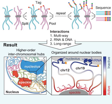
Eukaryotic genomes are packaged into a three-dimensional structure in the nucleus. Current methods for studying genome-wide structure are based on proximity-ligation. However, this approach can fail to detect known structures, such as interactions with nuclear bodies, because these DNA regions can be too far to directly ligate. Accordingly, our overall understanding of genome organization remains incomplete. Here, we develop Split-Pool Recognition of Interactions by Tag Extension (SPRITE), which enables genome-wide detection of higher-order interactions within the nucleus. Using SPRITE, we recapitulate known structures identified by proximity-ligation and identify additional interactions occurring across larger distances, including two hubs of inter-chromosomal interactions that are arranged around the nucleolus and nuclear speckles. We show that a substantial fraction of the genome exhibits preferential organization relative to these nuclear bodies. Our results generate a global model whereby nuclear bodies act as inter-chromosomal hubs that shape the overall packaging of DNA in the nucleus.
Graphical abstract
IN BRIEF: SPRITE is introduced as a method that enables genome-wide detection of multiple simultaneously occurring higher-order DNA interactions within the nucleus and provides a global picture of interchromosomal spatial arrangement around nuclear bodies
INTRODUCTION
Although the same genomic DNA is packaged in the nucleus of each cell, different sets of genes are expressed in different cell states. Despite significant progress over the past decade, there are still many unanswered questions about how the genome is organized within the nucleus and how these structures change across different cell states.
Current methods for genome-wide mapping of 3-dimensional (3D) genome structure rely on proximity ligation (e.g. Hi-C), which work by ligating the ends of DNA regions that are in close spatial proximity in the nucleus followed by sequencing to map pairwise interactions. These methods have shown that the genome is largely organized around chromosome territories, such that most DNA interactions occur within an individual chromosome (Gibcus and Dekker, 2013). These interactions include chromatin loops that connect genomic DNA regions such as enhancers and promoters, local interacting neighborhoods of DNA called topologically associated domains (TADs), and compartments where DNA regions interact based on transcriptional activity (Pombo and Dillon, 2015).
Another widely-used method for studying nuclear structure is microscopy, which involves in situ imaging of DNA, RNA, and protein in the nucleus. These methods have shown that specific regions of the genome, including specific inter-chromosomal interactions, can organize around nuclear bodies (Hu et al., 2010). For example, RNA Polymerase I transcribed ribosomal DNA (rDNA) genes, which are encoded on several distinct chromosomes, localize within the nucleolus (Pederson, 2011). In addition, specific examples of RNA Polymerase II (PolII) transcribed genes have been shown to localize near the periphery of nuclear speckles (Khanna et al., 2014), a nuclear body that contains various mRNA processing and splicing factors (Spector and Lamond, 2011). These observations, and others (Branco and Pombo, 2006; Lomvardas et al., 2006), demonstrate that genome interactions can occur beyond chromosome territories and organize around nuclear bodies.
Yet, despite the power of each of these methods for mapping nuclear structure, there is a growing appreciation that microscopy and proximity-ligation measure different aspects of genome organization (Giorgetti and Heard, 2016; Williamson et al., 2014). Specifically, microscopy measures the 3D spatial distances between DNA sites within single cells, whereas proximity-ligation measures the frequency with which two DNA sites are close enough in the nucleus to directly ligate (Dekker, 2016). This difference is particularly significant when considering DNA regions that organize around nuclear bodies, which can range in size from 0.5-2μm (Pederson, 2011), and therefore may be too far apart to directly ligate. This may explain why proximity-ligation methods do not identify known interactions between chromosomes that organize around specific nuclear bodies.
These differences between proximity-ligation and microscopy highlight a challenge for generating comprehensive maps of genome structure. Specifically, it remains unclear whether the specific inter-chromosomal interactions identified by microscopy represent special cases or broader principles of global genome organization. Additionally, both methods are limited to measuring simultaneous contacts between a small number (~2-3) of genomic regions and therefore cannot measure how multiple DNA sites simultaneously organize within the nucleus (O’Sullivan et al., 2013). Accordingly, current methods cannot generate a global picture of genome organization, which is critical for addressing key questions, such as why some specific PolII-transcribed regions associate with nuclear speckles while others do not (Shopland et al., 2003), which DNA regions organize simultaneously around the same nuclear body, and how genomic DNA is organized in the nucleus relative to multiple nuclear bodies, chromosome territories, and other features.
To address these technical challenges, we develop a method called Split-Pool Recognition of Interactions by Tag Extension (SPRITE) that moves away from proximity-ligation and enables genome-wide detection of multiple DNA interactions that occur simultaneously within the nucleus. Using SPRITE, we recapitulate known genome structures identified by Hi-C, including chromosome territories, compartments, topologically associated domains, and loop structures, and identify that many of these occur within higher-order structures in the nucleus. Because SPRITE does not rely on proximity-ligation, it identifies interactions that occur across larger spatial distances than can be observed by Hi-C. These long-range interactions include two major hubs of inter-chromosomal interactions. By extending SPRITE to simultaneously measure RNA and DNA interactions, we find that these two inter-chromosomal hubs correspond to DNA organization around the nucleolus and nuclear speckles, respectively. Moreover, DNA regions within these hubs can simultaneously organize around the same nuclear body within individual cells. We show that gene-dense and highly transcribed PolII regions organize around nuclear speckles and gene poor, and therefore transcriptionally inactive, regions that are centromere-proximal organize around the nucleolus. In addition to the regions that directly associate with these nuclear bodies, we find that a substantial fraction of the genome exhibits preferential spatial positioning relative to each of these nuclear bodies. Importantly, these preferential spatial distances quantitatively correspond to functional and structural properties, including the density of active PolII within a genomic region. Together, our results provide a global model of genome organization whereby nuclear bodies act as inter-chromosomal hubs that shape the overall 3D packaging of DNA in the nucleus.
RESULTS
SPRITE: A genome-wide method to identify higher-order DNA interactions in the nucleus
We sought to develop a genome-wide method that enables mapping of higher-order interactions that occur simultaneously between multiple DNA sites within the same nucleus. To do this, we developed SPRITE, a method that does not rely on proximity ligation. SPRITE works as follows: DNA, RNA, and protein are crosslinked in cells, nuclei are isolated, chromatin is fragmented, interacting molecules within an individual complex are barcoded using a split-pool strategy, and interactions are identified by sequencing and matching all reads that contain identical barcodes (Figure 1A, Methods).
Figure 1. SPRITE accurately maps known genome structures across various resolutions.
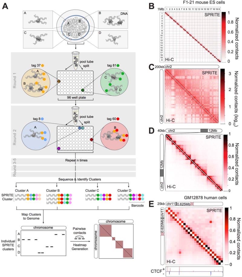
(A) Schematic of the SPRITE protocol. Crosslinked DNA is split into a 96-well plate and tagged with a unique sequence (colored circle) and then pooled into one tube. This split-and-pool process is repeated with tags sequentially added. DNA is sequenced, and tags are matched to generate SPRITE clusters. (B-D) Comparison of SPRITE (upper diagonal) and Hi-C (Dixon et al., 2012) (lower diagonal) in mouse embryonic stem cells (mESCs) (B) across all chromosomes at 1 Mb resolution, (C) on chromosome 2 at 200kb resolution (shown in log scale), and (D) within a 12 Mb region at 40 kb resolution. (E) Comparison of SPRITE and Hi-C (Rao et al., 2014) in human GM12878 cells within a 625 kb region at 25 kb resolution. CTCF binding (ENCODE) is colored based on motif orientation.
Specifically, we uniquely barcode each molecule in a crosslinked complex by repeatedly splitting all complexes across a 96-well plate (“split”), ligating a specific tag sequence onto all DNA molecules within each well (“tag”), and then pooling these complexes into a single well (“pool”). After several rounds of split-pool tagging, each molecule in an interacting complex contains a unique series of ligated tags, which we refer to as a barcode (Figure 1A). Because all molecules in a crosslinked complex are covalently linked, they will sort together in the same wells throughout each round of the split-pool tagging process and will contain the same barcode, whereas the molecules in separate complexes will sort independently and therefore will obtain distinct barcodes. Therefore, the probability that molecules in two independent complexes will receive the same barcode decreases exponentially with each additional round of split-pool tagging. For example, after 6 rounds of split-pool tagging, there are ~1012 possible unique barcode sequences, which exceeds the number of unique DNA molecules present in the initial sample (~109). After split-pool tagging, we sequence all tagged DNA molecules and match all reads with shared barcodes (Methods). We refer to all unique DNA reads that contain the same barcode as a SPRITE cluster (Figure 1A).
To confirm that DNA reads within a SPRITE cluster represent interactions that occur in the same nucleus and are not formed by spurious association or aggregation in solution, we mixed crosslinked lysates from human and mouse cells prior to performing SPRITE and found that ~99.8% of all SPRITE clusters contained only human or mouse reads, but not both (Methods, Figure S1A).
SPRITE differs from previous methods in several ways. In contrast to Hi-C, SPRITE can measure multiple DNA molecules that simultaneously interact within an individual nucleus, provides information about interactions that are heterogeneous from cell-to-cell, and is not restricted to measuring DNA interactions that are close enough in the nucleus to directly ligate. In contrast to Genome Architecture Mapping (GAM) (Beagrie et al., 2017), another proximity-ligation independent method, SPRITE can be performed without requiring specialized equipment or training, is faster to perform, and does not require extensive whole genome amplification. Furthermore, because SPRITE does not rely on proximity-ligation or whole genome amplification, it can be extended beyond DNA to directly incorporate RNA simultaneously. We describe these specific features of SPRITE in the following sections.
SPRITE accurately maps known genome structures across various resolutions
To test whether SPRITE can accurately map genome structure, we compared the results obtained by SPRITE to those measured by Hi-C. Specifically, we generated SPRITE maps in two mammalian cell types that have been previously mapped by Hi-C – mouse embryonic stem cells (mES) (Dixon et al., 2012) and human lymphoblastoid cells (GM12878) (Rao et al., 2014). We generated ~1.5 billion sequencing reads from each sample and matched reads containing the same barcode to obtain ~50 million SPRITE clusters from each sample (Methods). These SPRITE clusters range in size from 2 reads to >1000 reads per cluster (Figure S1C). To directly compare SPRITE and Hi-C, we converted SPRITE clusters into pairwise contact frequencies by enumerating all pairwise contacts observed within a single cluster and down-weighting each pairwise contact by the total number of molecules contained within the cluster (Figure 1A). This normalization prevents large SPRITE clusters from disproportionately impacting the pairwise frequency maps (Methods).
Overall, the pairwise contact maps generated with SPRITE are highly comparable to Hi-C maps, with similar structural features observed across all levels of genomic resolution. At a genome-wide level, we observe a clear preference for interactions that occur within the same chromosome (Figure 1B). At a chromosome-wide level, we observe similar A and B compartments as identified by Hi-C in both the mouse and human data (Spearman ρ= 0.85, 0.93, respectively) (Figure S1D-F). These correspond to locations of active and inactive transcription (Gibcus and Dekker, 2013). At 40kb resolution, we observe topologically associated domains (TADs), where adjacent DNA sites organize into highly self-interacting domains separated by boundaries that preclude interactions with other neighboring regions (Figure 1D). The location and strength of TAD boundaries, measured by insulation scores across the genome, are highly correlated in Hi-C and SPRITE for both mouse and human (Spearman ρ= 0.90, 0.94) (Figure S1G-I). Finally, at 25kb resolution, we observe specific “looping” interactions that connect local regions that contain the expected convergent CTCF motif orientation previously described for loop structures (Figure 1E, Figure S1J) (Sanborn et al., 2015). More generally, we find that the loops previously identified by Hi-C are strongly enriched within our SPRITE data at 10kb resolution (Figure S1K-L, Methods).
SPRITE identifies higher-order interactions that occur simultaneously
In addition to confirming pairwise genome structures identified by Hi-C, SPRITE can also directly measure multiple DNA regions that interact simultaneously within an individual cell, which we refer to as higher-order interactions. Although microscopy and specific proximity-ligation methods can also map higher-order interactions (Darrow et al., 2016; Olivares-Chauvet et al., 2016), these are largely restricted to mapping 3-way contacts. In contrast, SPRITE is not restricted in the number of simultaneous DNA contacts.
To explore the higher-order structures identified by SPRITE, we enumerated all interactions that occur simultaneously between 3 or more independent genomic regions (k ≥ 3), which we refer to as a k-mer. Similar to pairwise contact frequencies, one of the largest determinants of k-mer frequency in our data is the linear genomic distance separating each region in the k-mer. To account for this, we computed an enrichment score by normalizing the frequency of the observed k-mer by the average frequency observed across random k-mers that retain the same genomic distance (Figure S2A, Methods).
Overall, we identified >310,000 k-mers (1Mb resolution, k=3-14 regions) that were observed in at least 5 independent SPRITE clusters, occurred at a frequency that exceeded 90% of the random permutations, and occurred >4-fold more frequently than the average of the permuted regions (Figure S2B, Table S1A, Methods). Importantly, the frequency of observing even a single higher-order SPRITE cluster that does not represent a set of interactions that occur within the same individual cell is extremely low (<0.2% of all clusters, Figure S1A).
These enriched k-mers include various higher-order genomic DNA structures, including active compartments, gene clusters, and consecutive loop structures.
(i) Active Compartments
We observed highly enriched k-mers that connect multiple A compartment (transcriptionally active) regions that are non-contiguous and span large distances of the same chromosome. Specifically, we observed tens of thousands of individual SPRITE clusters that contain reads from at least three different A compartment regions that span at least 100 megabases within an individual chromosome (Table S1B-C, Figure 2A, S2C). This suggests that active DNA regions may interact within higher-order compartments (Figure 2B).
Figure 2. SPRITE identifies higher-order interactions that occur simultaneously.
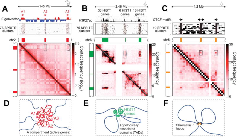
(A) Compartment eigenvector showing A (red) and B (blue) compartments on mouse chromosome 2 (Top). Individual SPRITE clusters (rows) containing reads mapping to at least 3 distinct regions (*) (Middle). Pairwise contact map at 200kb resolution (Bottom). (B) Schematic of multiple A compartment interactions. (C) H3K27ac ChIP-seq signal across a 2.46 Mb region on human chromosome 6 corresponding to 3 TADs containing 55 histone genes (Top). SPRITE clusters containing reads in all 3 TADs (Middle). Pairwise contact map at 25kb resolution (Bottom). (D) Schematic of higher-order interactions of HIST1 genes (green). (E) CTCF motif orientations at 3 loop anchors on human chromosome 8 (Top). SPRITE clusters overlapping all 3 loop anchors (Middle). Pairwise contact map at 25kb resolution (Bottom). (F) Schematic of higher-order interactions between consecutive loop anchors.
(ii) Gene Clusters
We identified >75 SPRITE clusters that connect three non-contiguous genomic regions within the human HIST1 cluster that encode 55 human histone genes (Figure 2C). Notably, these SPRITE clusters skip the intervening transcriptionally inactive regions. The frequency of SPRITE clusters that connect the three HIST1 gene clusters was never observed in any of the 100 randomly permuted k-mers containing the same genomic distance. This result suggests that multiple histone gene clusters simultaneously interact, consistent with observations that histone genes localize within specific nuclear bodies referred to as histone locus bodies (Nizami et al., 2010) (Figure 2D).
(iii) Consecutive Loops
Previous Hi-C studies suggested that consecutive loops may form higher-order interactions that bring together three distinct regions of the genome (Sanborn et al., 2015). Consistent with this, we observe several examples of highly enriched k-mers that correspond to consecutive loop structures (Figure S2D). For example, we observe >19 SPRITE clusters that contain reads corresponding to three loop anchor points on human chromosome 8 (Figure 2E). This suggests that multiple consecutive loops may occur simultaneously within the same cell (Figure 2F).
In addition to these examples, we also observe >11,000 enriched SPRITE k-mers corresponding to simultaneous 3-way interactions of TAD regions containing multiple enhancers and highly transcribed regions previously reported by GAM (Table S1D-E, Figure S2E). Taken together, these results suggest that SPRITE can detect multiple DNA interactions that occur simultaneously.
SPRITE identifies interactions that occur across large genomic distances
Because SPRITE does not rely on proximity ligation, which requires two DNA sites to be close enough to form a ligation junction (Dekker, 2016; Giorgetti and Heard, 2016), we reasoned that SPRITE might identify additional interactions that occur at further nuclear distances than those identified by Hi-C (Figure 3A). Indeed, we noticed that the number of pairwise contacts observed between two genomic regions as a function of their linear genomic distance (“distance decay”) occurs at different rates when comparing the Hi-C and SPRITE data (Figure S3A). Specifically, SPRITE identifies a significantly larger number of pairwise contacts that are present at larger linear genomic distances. Importantly, these additional long-range interactions correspond to an increased number of contacts between specific genomic regions expected to interact (Table S2A). For example, we observe a significant increase in interactions occurring between non-local active compartments separated by >100Mb (Figure S3B).
Figure 3. SPRITE identifies interactions across large genomic distances and across chromosomes.
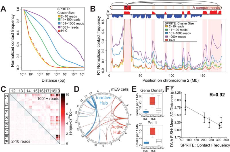
(A) Proximity ligation methods identify interactions that are close enough to directly ligate (green check), but miss those that are too far apart to ligate (red x). SPRITE identifies all crosslinked interactions within a complex and measures different DNA cluster sizes generated by fragmentation of the nucleus. (B) Relationship between contact frequency observed by Hi-C and different SPRITE cluster sizes relative to linear genomic distance in mESCs. (C) Contact frequency between a specific region (R1: 25-34 Mb) and other regions on mouse chromosome 2 for different SPRITE cluster sizes and Hi-C. Red shaded areas represent A compartment. (D) Interaction p-values are shown for SPRITE clusters of size 2-10 reads (lower diagonal) and 1001+ reads (upper diagonal) between mouse chromosomes 12 through 19. (E) Circos diagram of two sets of significant inter-chromosomal interactions are shown in blue (inactive hub) and red (active hub). (F) Box plots of gene density (left) and RNA polymerase II occupancy (right) for regions in the inactive hub (blue), active hub (red), or neither hub (grey).
Because SPRITE uses fragmentation to generate clusters of crosslinked interactions within the nucleus, we reasoned that small SPRITE clusters may represent interactions that are close in 3D space, whereas larger SPRITE clusters may represent interactions crosslinked across farther distances (Figure 3A). To test this, we stratified the SPRITE clusters based on their number of reads and generated pairwise contact maps. For small SPRITE clusters (2-10 reads), we observe a distance decay rate comparable to the rate observed by Hi-C, with most contacts occurring in close linear distances. Indeed, SPRITE clusters containing 2-10 reads also show pairwise contact maps that are similar to Hi-C (Figure S3C). In contrast, for the larger SPRITE clusters (11-1000+ reads), a larger number of contacts occur at longer genomic distances and the number of interactions at these longer distances increases with cluster size (Figure 3B). These different cluster sizes represent interactions that correspond to different structural features (Table S2A). For example, the small clusters preferentially identify interactions within TADs and within local compartment regions, while larger clusters correspond to increased interactions between distinct TADs as well as distal compartment regions (Figure 3C, S3C-D).
These results demonstrate that SPRITE captures longer-range interactions than are observed by Hi-C and that the distances that interactions occur can be measured using SPRITE clusters of different sizes (Figure 3A).
Inter-chromosomal interactions are partitioned into two distinct hubs
We also observed many inter-chromosomal interactions that are identified within the larger SPRITE clusters (11-1000+ reads), but are not observed in the smaller clusters or by Hi-C (Figure 3D, S3E-G).
To explore these inter-chromosomal interactions, we built a graph connecting all 1Mb regions in the mouse genome containing a significant pairwise interaction (p-value < 10−10) (Figure 3E). These interactions segregate into two discrete “hubs,” such that a large number of contacts occur within each hub, but no interactions occur between the two hubs. These hubs contain different functional properties: the first hub corresponds to gene-poor and therefore transcriptionally inactive regions, whereas the second hub corresponds to gene-dense regions that are highly transcribed by RNA polymerase II, enriched for active chromatin modifications, and contain other features of active transcription (Figure 3F, S3J, see Methods). Based on these properties, we refer to these hubs as the “inactive hub” and “active hub”, respectively (Table S2B-C).
Importantly, we observed two similar inter-chromosomal hubs in the human genome that displayed comparable functional properties (Figure S3K-N, Table S2D-E). Given the similar properties of the mouse and human hubs, we focused on mouse ES cells for our subsequent characterization of these hubs.
RNA-DNA SPRITE reveals that the inactive inter-chromosomal hub is organized around the nucleolus
To understand where in the nucleus these inter-chromosomal interactions occur, we first explored the inactive hub and noticed that several of the DNA regions in this hub are linearly close to genomic DNA regions that encode ribosomal RNAs (rDNA, see Methods). Because rDNA regions are known to be organized and transcribed within the nucleolus (Pederson, 2011), we hypothesized that the inactive hub regions may organize around the nucleolus.
To test this, we explored whether the DNA regions in this hub are associated with ribosomal RNA localization, which demarcates the nucleolus (Pederson, 2011). Specifically, we adapted the SPRITE protocol to enable simultaneous mapping of interactions between RNA and DNA molecules by ligating an RNA-specific adaptor that enable simultaneous tagging of both DNA and RNA during each round of the split-pool procedure (see Methods, Figure S4A-B). Using this approach, we mapped the interactions of ribosomal RNA on genomic DNA and found it was specifically enriched over the genomic DNA regions contained within the inactive hub (Figure 4A). In fact, ribosomal RNA enrichment across the genome is correlated with how frequently a region contacts the inactive hub (Figure 4A, S4C).
Figure 4. Genomic DNA in the inactive hub is organized around the nucleolus.
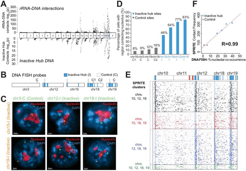
(A) Ribosomal RNA (rRNA) localization across the mouse genome identified using RNA-DNA SPRITE (top) compared to the DNA SPRITE contact frequency with regions in the inactive hub (bottom). (B) Locations of probe regions used for DNA FISH experiments. (C) Example images from immunofluorescence for nucleolin (red) combined with DNA FISH for six different pairs of DNA FISH probes (orange and green) and DAPI (blue). (D) Percent of cells that overlap nucleolin (distance = 0 μm) for 8 different probe regions, 4 control regions (grey) and 4 inactive hub regions (blue) measured in 50-155 cells/region. (E) Example of individual SPRITE clusters (rows) containing reads from different combinations of inactive hub regions (blue) on chromosomes 10, 12, 18 and 19 binned at 1Mb resolution. (F) Comparison of co-association of two DNA sites on different chromosomes around the same nucleolus measured by microscopy (x-axis) and SPRITE co-association frequency (y-axis) for six pairs of regions (see details in Figure S4F, n = 50-64 cells).
To confirm that the inactive hub represents DNA sites located near the nucleolus in situ, we performed DNA FISH combined with immunofluorescence for nucleolin, a protein marker of the nucleolus. Specifically, we selected DNA FISH probes for 4 genomic regions in the inactive hub and 3 control regions on the same chromosomes. We selected an additional control region on a chromosome lacking any inactive hub regions (Figure 4B). We calculated the 3D distance between each allele and the nearest nucleolus and found that inactive hub regions are dramatically closer to the nucleolus than negative control regions (average ~750nm closer, Figure S4D). In the majority of cells analyzed, at least one allele of the inactive hub DNA regions directly contacts the periphery of the nucleolus (~61% of cells, Figure 4C-D, Figure S4D-E). Therefore, we refer to this hub as the nucleolar hub. Our results confirm previous observations that the nucleolus can act as an anchor for inactive chromatin regions (Padeken and Heun, 2014).
Because many genomic regions are contained within the nucleolar hub, we hypothesized that multiple DNA sites simultaneously interact around a single nucleolus. Consistent with this, we observed >1,200 SPRITE clusters that contain simultaneous interactions between at least three distinct genomic regions on different chromosomes in the nucleolar hub (Figure 4E, Table S3). To confirm these inter-chromosomal contacts occur through co-localization at the same nucleolus, we performed 2-color DNA FISH combined with immunofluorescence for nucleolin and measured the frequency of co-association at the same nucleolus (Movie S1). We observed that two regions in the nucleolar hub were ~7-times more likely to co-occur around the same nucleolus compared to a nucleolar hub region and control region (Figure S4F). Importantly, the frequency of co-occurrence of a pair of DNA sites at the same nucleolus measured by microscopy is highly correlated with the frequency at which these genomic DNA regions co-occur within the same SPRITE clusters (Pearson r=0.99, Figure 4F). This demonstrates that SPRITE quantitatively measures the frequency at which DNA sites co-occur at a nuclear body within single cells.
Together, these results provide a genome-wide map of DNA regions that spatially organize around the nucleolus. While other studies have previously mapped individual regions that contact the nucleolus across a population of cells (Németh et al., 2010), our results provide a genome-wide 3D picture of how multiple DNA sites arrange simultaneously around the nucleolus.
The active inter-chromosomal hub is organized around nuclear speckles
We noticed that the genomic DNA regions within the active hub are strongly enriched for U1 spliceosomal RNA and Malat1 lncRNA localization (Engreitz et al., 2014) (Figure S5A) and the level of their localization is highly correlated with how frequently a DNA region interacts with the active hub (Spearman ρ =0.80 and 0.74, Figure 5A, S5B). Because the U1 and Malat1 RNAs are known to localize at nuclear speckles (Hutchinson et al., 2007), a nuclear body that contains proteins involved in mRNA splicing and processing (Spector and Lamond, 2011), we hypothesized that inter-chromosomal interactions occurring between regions in the active hub may be spatially organized around nuclear speckles.
Figure 5. Genomic DNA in the active hub is organized around nuclear speckles.
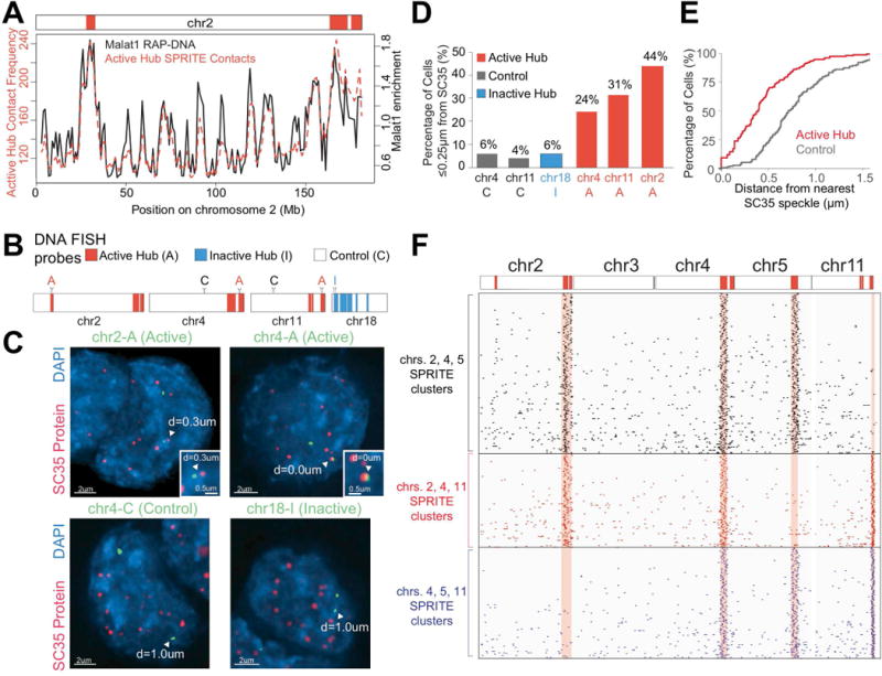
(A) Malat1 lncRNA localization (black) (Engreitz et al., 2014) compared to SPRITE contact frequency with regions in the active hub (red). (B) Locations of probe regions used for DNA FISH experiments. (C) Example images from immunofluorescence for SC35 (red) combined with DNA FISH for six DNA regions (green) and DAPI (blue) performed in formaldehyde fixed cells. Arrowhead: 3D distance to SC35 is noted. (D) Percentage of cells with at least 1 allele within 0.25 μm of SC35 (n = 41-90 cells). See Figure S5E for further quantitation. (E) Cumulative frequency of minimum 3D distance to SC35 for active hub (red) and control (grey) regions. (F) Example individual SPRITE clusters (rows) containing reads from different combinations of 3 active hub regions on chromosomes 2, 4, 5 and 11. (G) Images of 2 active hub regions on different chromosomes that are close to the same nuclear speckle.
To test this, we performed DNA FISH combined with immunofluorescence for SC35, a well-known protein marker of nuclear speckles. We selected FISH probes targeting 3 DNA regions contained in the active hub and 2 control regions on the same chromosome not in the active hub. We also selected another control region within the inactive hub (Figure 5B). We calculated the 3D distance between each region and the closest nuclear speckle and found that all 3 active hub regions are consistently closer to nuclear speckles compared with the 3 control regions (Figure 5C-E, S5C-G). Indeed, for active hub regions, we observe a dramatic increase in the number of cells where at least one allele directly touches a nuclear speckle relative to control regions (~13-fold, Figure S5G). Despite this preferential organization near the nuclear speckle, the number of cells in which an active region directly contacts the nuclear speckle is relatively low (~10% of cells), which is consistent with previous observations by live-cell microscopy that individual genomic DNA interactions with a nuclear speckle are transient (Khanna et al., 2014). Based on these observations, we refer to the DNA regions in this hub as the nuclear speckle hub.
We hypothesized that nuclear speckle hub regions may simultaneously organize around the same nuclear speckle. Indeed, we identified >690 SPRITE clusters containing at least three distinct active hub regions that were present on different chromosomes (Table S4, Figure 5F). Consistent with this, we observe two DNA sites in the speckle hub are >8-times as likely to be within 1μm of each other by microscopy compared to an active and control region (Figure S5H). Indeed, we observe two pairs of genomic DNA regions in the active hub preferentially organized near the same nuclear speckle in 2 out of 15 cells that were measured (Figure 5G). In contrast, we did not observe even a single example of an active hub and control region that were organized near the same speckle in 21 cells that were measured. However, because there are many nuclear speckles in a given cell (~20/nucleus) and DNA interactions with an individual nuclear speckle can be transient (~10% of regions directly contact any speckle), it is challenging to robustly quantify the frequency at which multiple DNA regions simultaneously associate around the same nuclear speckle using microscopy (see Methods).
Our results confirm previous observations that specific actively transcribed regions can interact with nuclear speckles (Brown et al., 2008; Khanna et al., 2014; Shopland et al., 2003) and extend this observation genome-wide by providing a map of DNA interactions around nuclear speckles. Moreover, our results suggest that multiple actively transcribed DNA regions can arrange simultaneously around nuclear speckles to form higher-order inter-chromosomal interactions.
Nuclear bodies constrain the overall 3D organization of genomic DNA in the nucleus
We considered that nuclear bodies might play an important role in defining the overall arrangement of genomic DNA in the nucleus because they organize large hubs of inter-chromosomal interactions. To address this, we focused on how genomic regions that are not within these hubs are spatially positioned relative to each nuclear body. We considered 3 possibilities: these regions show (i) random spatial positioning with respect to either nuclear body (random preference), (ii) spatial positioning that linearly decays as a function of genomic distance from a hub-associated region (linear preference), or (iii) specific non-linear spatial preferences to either nuclear body (non-linear preference).
To test these possibilities, we calculated the average number of SPRITE contacts for each 1Mb region in the genome relative to regions in the nucleolar or nuclear speckle hubs (Figure 6A). Interestingly, we find that a large fraction of genomic regions exhibit preferential contacts with either hub (Figure 6A), such that regions that frequently contact the nucleolar hub are depleted relative to the nuclear speckle hub, and vice versa (Figure 6B). Importantly, these preferential contacts do not occur exclusively at regions in close linear distance to hub regions, as would be expected if this organization occurred through a linear “dragging” effect of the chromatin polymer. For example, several non-contiguous regions on mouse chromosome 11 have high speckle hub contact frequencies despite being linearly far from speckle hub regions (Figure 6B). Moreover, several non-contiguous genomic regions preferentially contact the nucleolar hub even though chromosome 11 does not contain any nucleolar hub regions (Figure 6B). These results suggest that a large fraction of genomic DNA regions show preferential non-linear spatial arrangement to either the nucleolus or nuclear speckle.
Figure 6. Preferential DNA distance to the nucleolus and nuclear speckles constrain overall genome organization.
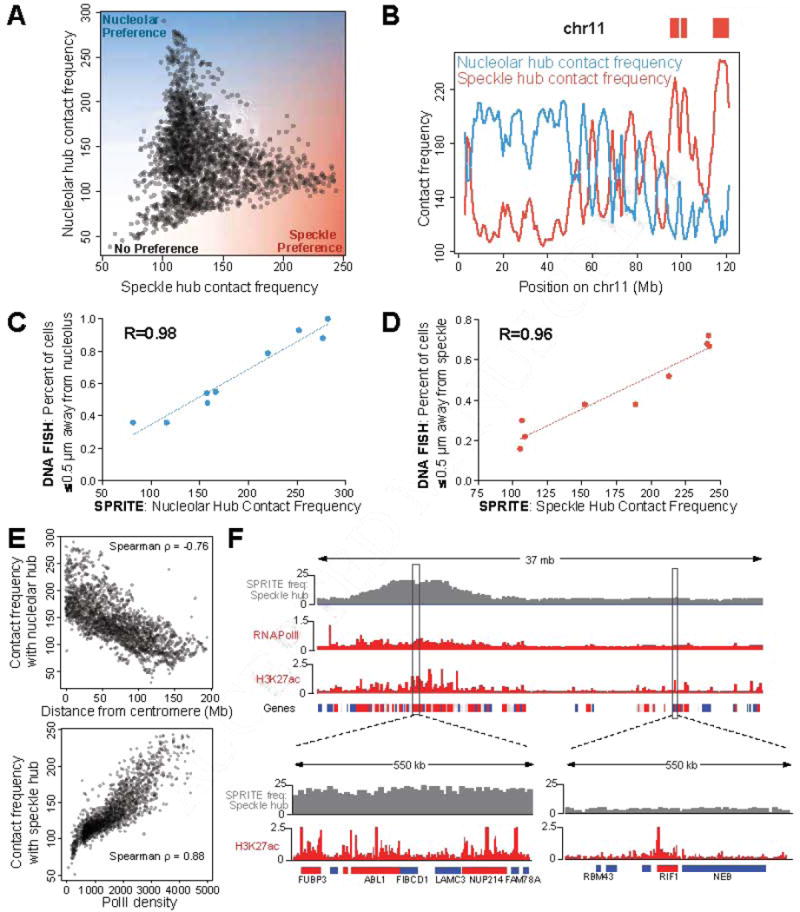
(A) SPRITE contact frequency to the nucleolar hub (y-axis) or speckle hub (x-axis) for each 1Mb genomic bin in mES cells. (B) SPRITE contact frequency to the nucleolar hub (blue) or speckle hub (red) across mouse chromosome 11. Red boxes represent active hub regions. (C) SPRITE contact frequency to the nucleolar hub (x-axis) compared to DNA FISH contact frequency to the nucleolus as measured by microscopy across 50-155 cells/region (y-axis). (D) SPRITE contact frequency to the speckle hub (x-axis) compared to DNA FISH contact frequency to nuclear speckles as measured by microscopy (y-axis) across 50-51 cells/region. See Figure S6B-D for further details. (E) SPRITE contact frequencies with the nucleolar hub (y-axis) and centromere distance (x-axis) (top) and SPRITE contacts with the speckle hub (y-axis) and PolII density (x-axis, ENCODE) (bottom). (F) SPRITE contact frequency with the speckle hub compared to RNA PolII and H3K27ac signal (ENCODE) across a region on chromosome 2. Highly expressed (red, FPKM>10), moderately expressed (grey FPKM=2-10), or inactive (blue, FPKM=0-2) genes are indicated. Zoom-in: chr2:31.4-30.0 Mb (left) and chr2:51.7-52.3 Mb (right).
To confirm that these spatial preferences accurately represent 3D distances of DNA sites to these nuclear bodies in situ, we performed DNA FISH combined with immunofluorescence for nucleolin or SC35. Specifically, we selected 9 DNA regions across a range of SPRITE contact frequencies relative to the nucleolus, including nucleolar hub regions, a speckle hub region, and 4 regions with different intermediate spatial preferences (Figure S6B-C). In all cases, the 3D distances between each DNA region and the nucleolus is strongly correlated with its SPRITE contact frequency to the nucleolar hub (Pearson r = 0.98, Figure 6C, S6D). Similarly, we selected 9 DNA regions across a range of SPRITE contact frequencies relative to the speckle hub, including speckle hub regions, a nucleolar hub region, and 3 regions with different intermediate spatial preferences (Figure S6B-C). The 3D distance between each DNA region and a nuclear speckle is strongly correlated with its SPRITE contact frequency to the nuclear speckle hub (Pearson r = 0.98, Figure 6D, S6B-D). These results demonstrate that SPRITE provides accurate quantitative measurements of 3D spatial distances across the nucleus.
Functional and structural properties define preferential organization to nuclear bodies
To understand the basis of these spatial preferences, we examined the structural and functional properties of the DNA regions positioned close to each nuclear body.
(i) Nucleolar preference
We found that regions that are linearly close to the centromere are closer to the nucleolus (Figure 6E, Spearman ρ = 0.76). Notably, these results are consistent with previous observations that centromeres often co-localize on the periphery of the nucleolus (Pollock and Huang, 2009; Tjong et al., 2016) Figure S7A-B). However, not all genomic regions close to centromeres are close to the nucleolus because actively transcribed regions are excluded from the nucleolar compartment even when they reside in linear proximity to a centromere (Figure S6E). Because actively transcribed regions are preferentially positioned away from the nucleolus, the genomic DNA regions that are closer to the nucleolus tend to correspond to inactive chromatin (Figure S6A,E).
Importantly, not all inactive regions are positioned close to the nucleolus, they can also arrange close to the nuclear lamina (Peric-Hupkes et al., 2010). Given that the nuclear lamina is another nuclear structure known to organize inactive chromatin, we explored whether lamina-associated DNA regions form preferential interactions. Indeed, we observe an increased number of DNA contacts between genomic regions associated with the nuclear lamina; however, these lamina-associated interactions generally occur between regions that are linearly close to each other rather than between chromosomes (Figure S7C-D). Although both compartments are associated with inactive chromatin, we do not observe a global relationship between genomic regions that are close to the nucleolar hub and regions that are associated with the nuclear lamina (Figure S7E, spearman ρ = 0.01). In contrast, regions that are closer to the nuclear speckle are highly depleted for nuclear lamina association (Spearman ρ = −0.71, Figure S7F).
(ii) Nuclear Speckle preference
Regions that are closer to nuclear speckles are strongly associated with high levels of active PolII transcription (Spearman ρ = 0.88, Figure 6E, S6F, Methods). Yet, we find that the transcriptional activity of an individual gene alone does not explain its distance to nuclear speckles because genomic DNA regions that are not transcribed, but are contained within highly transcribed gene-dense regions, tend to be closer to nuclear speckles (Figure 6F). Conversely, highly transcribed genes within otherwise inactive genomic regions tend to be farther from nuclear speckles (Figure 6F). These results demonstrate that the density of PolII transcription within a genomic neighborhood, rather than transcriptional activity of individual genes, defines proximity to nuclear speckles. This explains why only some of the specific actively transcribed genes previously studied organize close to nuclear speckles (Shopland et al., 2003) and may explain previous observations that actively transcribed gene-dense regions can “loop out” from the core chromosome territory (Branco and Pombo, 2006; Mahy et al., 2002).
Together, our results provide a global picture of the structural and transcriptional properties that define spatial positioning relative to nuclear bodies within the nucleus (Figure 7).
Figure 7. A global model for how nuclear bodies shape overall three-dimensional genome organization in the nucleus.
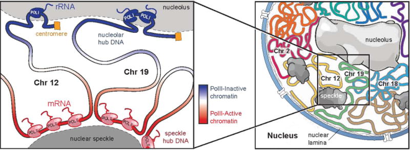
Left Panel: DNA regions containing a high-density of PolII associate with the nuclear speckle, while genomic regions linearly close to ribosomal DNA or centromeric regions associate with the nucleolus. This leads to co-association of multiple DNA regions around the same nuclear body to create spatial hubs of inter-chromosomal contacts. In addition to the genomic regions directly associating around these nuclear bodies, other DNA regions exhibit preferential organization, such that regions with higher levels of PolII density are closer to the nuclear speckle (red gradient) and regions with lower levels of PolII density are closer to the nucleolus (blue gradient). Right panel: These overall constraints act to shape the global layout of genomic DNA in the nucleus. DNA regions on the same chromosome tend to be closer to each other (colored lines). Yet, regions on different chromosomes containing similar properties organize around a nuclear body and can be closer to each other than to other regions contained on the same chromosome.
DISCUSSION
An integrated model of how the genome is packaged in the nucleus
We described SPRITE, a method that enables genome-wide mapping of higher-order DNA interactions that occur simultaneously within the nucleus. SPRITE fills a critical gap among current methods by bridging the information derived from microscopy with the ability to generate high-resolution genome-wide maps. In doing so, SPRITE provided new biological insights into how DNA is packaged in the nucleus at multiple levels.
Molecular Insights
SPRITE provides a genome-wide molecular picture of all DNA regions that contact specific nuclear bodies. These results confirm previous observations made by microscopy for a limited number of DNA regions (Brown et al., 2008) and extends this molecular picture genome-wide and at higher-resolution. This explains why some, but not other, active PolII-transcribed regions are organized around nuclear speckles and why some, but not other, inactive regions are organized around the nucleolus.
Spatial Insights
SPRITE provides a genome-wide spatial picture of how multiple DNA regions organize around the same nuclear body. This extends previous observations of a small number of specific DNA regions that can organize simultaneously around the same nuclear bodies (Brown et al., 2008; Strongin et al., 2014) to a global spatial picture where DNA organization around nuclear bodies form large spatial hubs of higher-order inter-chromosomal contacts.
Quantitative Global Insights
SPRITE provides a quantitative map of where DNA regions are organized relative to nuclear bodies, structural features, and other genomic regions. Specifically, we uncover quantitative preferences that spatially relate all genomic DNA regions to each nuclear body. Our results indicate that organization around nuclear bodies act as a dominant feature of global genome organization where: (i) a significant proportion of the genome preferentially organizes closer to one of these nuclear bodies and that (ii) organization around these bodies can lead to closer spatial organization of regions on different chromosomes. Because these spatial preferences correspond to PolII-transcriptional status, they may be dynamic between cell states.
Together, these results suggest an integrated and global picture of genome organization where individual genomic regions across chromosomes organize around nuclear bodies to shape the overall packaging of genomic DNA in a highly regulated and dynamic manner (Figure 7).
Although it remains unclear whether spatial organization around nuclear bodies directly impacts transcription or whether it is a consequence of PolII-occupancy within a genomic region, spatial segregation may provide regulatory advantages by segregating factors into regions of high local concentration within the nucleus. For example, organization of DNA near nuclear speckles could increase the efficiency of post-transcriptional mRNA processing by concentrating splicing and processing factors, which are enriched in the nuclear speckles, near actively transcribed genes. Future work will be needed to determine how this spatial organization is established, its functional role, and its dynamics across cell states.
SPRITE provides a powerful method for studying 3-dimensional spatial organization
This global model represents just one example of how SPRITE can be used to uncover new aspects of 3D genome organization in the nucleus. SPRITE provides several features that make it a powerful tool that can be applied to explore many open questions regarding organization and function in the nucleus.
Higher-order spatial interactions
SPRITE provides a genome-wide map of higher-order interactions that occur simultaneously in 3D spatial proximity within an individual nucleus. In contrast to proximity-ligation and microscopy methods, SPRITE is not limited in the number of simultaneous interactions that can be measured. This will enable exploration of additional higher-order interactions, such as spatial clusters of individual genes (e.g. olfactory receptor genes (Lomvardas et al., 2006)) and multiple enhancers that simultaneously interact with a promoter.
Global spatial maps
SPRITE accurately measures 3D spatial distances across a wide-range of nuclear distances. Because SPRITE does not rely on proximity-ligation, it is not restricted to identifying interactions between molecules that are close enough to directly ligate. This ability to measure longer-range distances and the ability to measure crosslinked complexes of different sizes, enables quantitative and global reconstruction of 3D spatial distances across the nucleus.
Simultaneous RNA and DNA maps
SPRITE is not restricted to measuring DNA molecules, but can also simultaneously map RNA within crosslinked complexes. Because RNA demarcates various nuclear bodies, including the nucleolus and nuclear speckles, this allowed us to define specific DNA hubs as organizing around these bodies. SPRITE can be extended to include direct measurements of additional RNAs to enable direct mapping of genome structure relative to other RNA-demarcated structures (Rinn and Guttman, 2014) as well as for exploring enhancer-promoter interactions and their corresponding nascent transcription levels.
More generally, SPRITE represents a powerful new framework for spatial mapping because it provides genome-wide data that is highly analogous to microscopy and can be used to explore large numbers of high resolution interactions that occur simultaneously in 3D space. Beyond its current applications, SPRITE can be extended in several ways. For example, SPRITE can be used to measure other spatial interactions beyond the nucleus, such as preferential associations of RNA in the cytoplasm (e.g. RNA phase separated bodies (Decker and Parker, 2012)). Furthermore, SPRITE can be extended to incorporate protein localization using pools of barcoded antibodies (Frei et al., 2016) to generate combinatorial and spatial maps of DNA, RNA, and/or protein. In addition, SPRITE can be extended to generate global single-cell maps by split-pool tagging of all molecules within individual cells (Ramani et al., 2017). These applications will enable exploration of previously inaccessible questions regarding the relationship between 3D genome structure and gene regulation within the nucleus and their dynamics across time.
STAR METHODS
CONTACT FOR REAGENT AND RESOURCE SHARING
Further information and requests for resources and reagents should be directed to and will be fulfilled by the Lead Contact, Mitchell Guttman (mguttman@caltech.edu).
EXPERIMENTAL MODEL AND SUBJECT DETAILS
Cell culture and lines used in analysis
Mouse ES cell lines were cultured in serum-free 2i/LIF medium and maintained at an exponential growth phase as previously described (Engreitz et al., 2014). SPRITE DNA-DNA maps were generated in female ES cells (F1 2-1 line, provided by K. Plath), a F1 hybrid wild-type mouse ES cell line derived from a 129 × castaneous cross. SPRITE RNA-DNA maps were generated in the pSM33 ES cell line (provided by K. Plath), a male ES cell line derived from the V6.5 ES cell line, which expresses Xist from the endogenous locus under the transcriptional control of a tet-inducible promoter and the Tet transactivator (M2rtTA) from the Rosa26 locus. We induced Xist expression in these cells using doxycycline (Sigma, D9891) at a final concentration of 2 μg/mL for 6-24 hours.
Human GM12878 cells, a female lymphoblastoid cell line obtained from Coriell Cell Repositories, were cultured in RPMI 1640 (Gibco, Life Technologies), 2 mM L-glutamine, 15% fetal bovine serum (FBS; Seradigm), and 1X penicillin-streptomycin and maintained at 37°C under 5% CO2. Cells were seeded every 3-4 days at 200,000 cell/mL in T25 flasks, maintained at an exponential growth phase, and passaged or harvested before reaching 1,000,000 cell/mL.
HEK293T, a female human embryonic kidney cell line transformed with the SV40 large T antigen was obtained from ATCC and cultured in complete media consisting of DMEM (Gibco, Life Technologies) supplemented with 10% FBS (Seradigm Premium Grade HI FBS, VWR), 1X penicillin-streptomycin (Gibco, Life Technologies), 1X MEM non-essential amino acids (Gibco, Life Technologies), 1 mM sodium pyruvate (Gibco, Life Technologies) and maintained at 37°C under 5% CO2. For maintenance, 800,000 cells were seeded into 10 mL of complete media every 3-4 days in 10 cm dishes.
METHOD DETAILS
Split-Pool Recognition of Interactions by Tag Extension (SPRITE)
Crosslinking
Cells were crosslinked in a single-cell suspension to ensure that we obtain individual crosslinked nuclei rather than crosslinked colonies of cells. GM12878 lymphoblast cells, which are grown in suspension, were pelleted and media was removed prior to crosslinking. Mouse ES cells, which are adherent, were trypsinized to remove from plates prior to crosslinking in suspension. Specifically, 5 mL of TVP (1 mM EDTA, 0.025% Trypsin, 1% Sigma Chicken Serum; pre-warmed at 37°C) was added to each 15 cm plate, then rocked gently for 3-4 minutes until cells start to detach from the plate. Afterwards, 25 mL of wash solution (DMEM/F-12 supplemented with 0.03% Gibco BSA Fraction V, pre-warmed at 37°C) was added to each plate to inactivate the trypsin. Cells were lifted into a 15 mL or 50 mL conical tube, pelleted at 330 g for 3 minutes, and then washed in 4 mL of 1X PBS per 10 million cells. During all crosslinking steps and washes, volumes were maintained at 4 mL of buffer or crosslinking solution per 10 million cells. After pelleting, cells were pipetted to disrupt clumps of cells and crosslinked in suspension with 4 mL of 2 mM disuccinimidyl glutarate (DSG, Pierce) dissolved in 1X PBS for 45 minutes at room temperature. DSG was removed, and cells were pelleted (as above) and washed with 1X PBS. A solution of 3% formaldehyde (FA Ampules, Pierce) in 1X PBS was added to cells for 10 minutes at room temperature. Formaldehyde was immediately quenched with addition of 200 μl of 2.5 M glycine per 1 mL of 3% FA solution. Cells were pelleted, formaldehyde was removed, and cells were washed three times with 0.5% BSA in 1X PBS that was kept at 4°C. Aliquots of 10 million cells were allocated into 1.7 mL tubes and pelleted. Supernatant was removed and cells were flash frozen in liquid nitrogen and stored in −80°C until lysis.
Chromatin Isolation
Crosslinked cell pellets (10 million cells) were lysed using the nuclear isolation procedure previously described in the HT-ChIP protocol. Specifically, cells were incubated in 1 mL of Nuclear Isolation Buffer 1 (50 mM Hepes pH 7.4, 1 mM EDTA pH 8.0, 1 mM EGTA pH 8.0, 140 mM NaCl, 0.25% Triton-X, 0.5% NP-40, 10% Glycerol, 1X PIC) for 10 minutes on ice. Cells were pelleted at 850 g for 10 minutes at 4°C. Supernatant was removed, 1 ml of Lysis Buffer 2 (50 mM Hepes pH 7.4, 1.5 mM EDTA, 1.5 mM EGTA, 200 mM NaCl, 1X PIC) was added and incubated for 10 minutes on ice. Nuclei were obtained after pelleting and supernatant was removed (as above), and 550 μL of Lysis Buffer 3 (50 mM Hepes pH 7.4, 1.5 mM EDTA, 1.5 mM EGTA, 100 mM NaCl, 0.1% sodium deoxycholate, 0.5% NLS, 1X PIC) was added and incubated for 10 minutes on ice prior to sonication.
Chromatin Digestion
After nuclear isolation, chromatin was digested via sonication of the nuclear pellet using a Branson needle-tip sonicator (3 mm diameter (1/8” Doublestep), Branson Ultrasonics 101-148-063) at 4°C for a total of 1 minute at 4-5 W (pulses of 0.7 seconds on, followed by 3.3 seconds off). DNA was further digested using 2-6 μL of TurboDNAse (Ambion) per 10 μL of sonicated lysate (equivalent to ~200,000 cells), in 1x DNase Buffer (Diluted from 10x DNase Buffer: 200 mM Hepes pH 7.4, 1 M NaCl, 0.5% NP-40, 5 mM CaCl2, 25 mM MnCl2) at 37°C for 20 minutes. Concentrations of DNase were optimized to obtain DNA fragments of approximately 150-1000 bp in length, which is needed for sequencing. DNAse activity was quenched by adding 10 mM EDTA and 5 mM EGTA.
Estimating molarity
After DNAse digestion, crosslinks were reversed on approximately 10 μl of lysate in 82 μL of 1X Proteinase K Buffer (20 mM Tris pH 7.5, 100 mM NaCl, 10 mM EDTA, 10 mM EGTA, 0.5% Triton-X, 0.2% SDS) with 8 μL Proteinase K (NEB) at 65°C overnight. The DNA was purified using Zymo DNA Clean and Concentrate columns per the manufacturer’s specifications with minor adaptations, such as binding to the column with 7X Binding Buffer to improve yield. Molarity of the DNA was calculated by measuring the DNA concentration using the Qubit Fluorometer (HS dsDNA kit) and the average DNA sizes were estimated using the Agilent Bioanalyzer (HS DNA kit).
NHS bead coupling
We used these numbers to calculate the total number of DNA molecules per microliter of lysate. We coupled the lysate to NHS-activated magnetic beads (Pierce) overnight at 4°C in 1 mL of 0.1% SDS in 1X PBS rotating on a HulaMixer Sample Mixer (Thermo). Specifically, we coupled 1x10¹⁰ DNA molecules to 1.75 mL of beads (mouse) and 5x10¹⁰ DNA molecules to 2 mL of beads (human). We obtain roughly 50% coupling efficiency of molecules to the beads, which effectively halves the ratio of molecules coupled per bead. This coupling ratio was selected to ensure that most beads contained less than 0.125 to 0.25 complexes per bead to reduce the probability of simultaneously coupling multiple independent complexes to the same bead, which would lead to their association during the split-pool barcoding process. At this loading concentration of 0.125 complexes per bead, we find that <0.2% of SPRITE clusters contain any inter-species contacts and <0.1% of pairwise contacts contain any spurious pairing of human and mouse fragments that arise due to bead coupling (Figure S1A).
After coupling lysate to NHS beads overnight, we quench the beads with 1 mL of 0.5 M Tris pH 8.0 for 1 hour at 4°C rotating on a HulaMixer. We then wash the beads four times at 4°C in 1mL of Modified RLT Buffer (1X Buffer RLT supplied by Qiagen with added 10 mM Tris pH 7.5, 1 mM EDTA, 1 mM EGTA, 0.2% NLS, 0.1% Triton-X, 0.1% NP-40) for 3 minutes each. Next, beads are washed in 1 mL of SPRITE Wash Buffer (1X PBS, 5 mM EDTA, 5 mM EGTA, 5 mM DTT, 0.2% Triton-X, 0.2% NP-40, 0.2% sodium deoxycholate) twice at 50°C and once at room temperature for 5 minutes each. These washes remove any material that is not covalently attached to the beads. Prior to performing all enzymatic steps, buffer is exchanged on the beads through two rinses using 1 mL of SPRITE Detergent Buffer (20 mM Tris pH 7.5, 50 mM NaCl, 0.2% Triton-X, 0.2% NP-40,0.2% sodium deoxycholate). These detergents are used throughout the protocol to prevent bead aggregation, which could result in spurious interactions. Because the crosslinked complexes are immobilized on NHS magnetic beads, we can perform several enzymatic steps by adding buffers and enzymes directly to the beads and performing rapid buffer exchange between each step on a magnet. All enzymatic steps were performed with shaking at 1200 rpm (Eppendorf Thermomixer) to avoid bead settling and aggregation, and all enzymatic steps were inactivated by adding 0.5-1 mL Modified RLT Buffer to the NHS beads.
DNA Repair
We then repair the DNA ends to enable ligation of tags to each molecule. Specifically, we blunt end and phosphorylate the 5′ ends of double-stranded DNA using two enzymes. First, T4 Polynucleotide Kinase (NEB) treatment is performed at 37°C for 1 hour, the enzyme is quenched using 1 mL Modified RLT buffer, and then buffer is exchanged with two washes of 1 mL SPRITE Detergent Buffer to beads at room temperature. Next, the NEBNext End Repair Enzyme cocktail (containing T4 DNA Polymerase and T4 PNK) and 1x NEBNext End Repair Reaction Buffer is added to beads and incubated at 20°C for 1 hour, and inactivated and buffer exchanged as specified above. DNA was then dA-tailed using the Klenow fragment (5′-3′ exo-, NEBNext dA-tailing Module) at 37°C for 1 hour, and inactivated and buffer exchanged as specified above.
Split-pool ligation
The beads were then repeatedly split-and-pool ligated over five rounds with a set of “DNA Phosphate Modified” (DPM), “Odd”, “Even” and “Terminal” tags (see SPRITE Tag Design below for details). The DPM tag is ligated by an “Odd” tag. The “Odd” and “Even” tags were designed so that they can be ligated to each other over multiple rounds, such that after Odd is ligated, then Even ligates the Odd tags, and then Odd can ligate the Even tags. This can be repeated such that the same two plates of tags can be used over multiple rounds of split-pool tagging without self-ligation of the adaptors to each other. Finally, a set of barcoded Terminal tags are ligated at the end to attach an Illumina sequence for final library amplification. In this study, we performed five rounds total of split-and-pool ligation in the following order: DPM, Odd, Even, Odd, and Terminal tag. Over each round, the samples are split across a 96-well plate in 4.4 μL of SPRITE Detergent Buffer per well to prevent aggregation of beads, which would result in spurious interactions. Each plate contained 2.4 μL of 96 different tags at a concentration of 45 μM. 10 μL of 2X Instant Sticky End Ligation Master Mix (NEB) and 3.2 μL of Ultra Pure H2O (Invitrogen) was added to each well of the 96-well plate, for a final concentration of 1X Instant Sticky End Ligation Master Mix per well. All ligations were performed at 20°C for 1 hour with shaking at 1600 rpm for 30 seconds every 5 minutes. Following every round of split-pool ligation, we inactivated the ligase via addition of 60 μL of Modified RLT Buffer to every well, which prevents spurious ligation of tags in the pooled tube. The sample was then pooled into a single 1.7 mL tube. After removing Modified RLT Buffer from the beads, remaining free tags were removed by washing the beads in 1 mL SPRITE Wash Buffer three times at 45°C for 3 minutes each. We then performed buffer exchange into SPRITE Detergent Buffer by adding 1 mL of Buffer and exchanging three times. We ensured that the majority of DNA molecules within a crosslinked complex are barcoded by optimizing the ligation efficiency such that >90% of DNA molecules are ligated during each round of split-pool tagging (Figure S1B).
Estimating sequencing depth
SPRITE interactions are defined based on the sequences that share the same tags. Accordingly, it is essential to sequence as many of the barcoded molecules in a complex as possible in order to identify interactions. Therefore, the number of unique molecules that are sequenced dramatically affects the likelihood of identifying interacting molecules. To address this, we optimized the loading density of our sequencing sample based on the number of unique molecules contained in the sample. Our goal is to load approximately equimolar unique molecules as the number of sequencing reads available. Specifically, based on our simulations, we have found that sequencing with ~1-3X coverage of reads per the number of unique molecules will ensure that most molecules are sampled. This follows Poisson sampling where 1-1/ec of molecules are sampled at a given c coverage. For example, 3X, 2X, and 1X coverage samples approximately 95%, 86%, and 63% of interactions, respectively. In this study, most libraries were sampled with approximately 1.5-2X coverage.
To estimate the number of unique molecules in our sample, we measure the amount of material present on beads prior to reverse crosslinking all interactions. To do this, we take an aliquot of the sample and reverse crosslink to elute (as above) the DNA, which is then cleaned and amplified for 9-12 cycles. We then measure the molarity using the Qubit and Bioanalyzer (as above). The number of unique molecules in the aliquot prior to amplification is back calculated from a standard curve and adjusted to account for loss during the cleanup. This is used to estimate the number of unique molecules in the remaining crosslinked sample. In addition to optimizing molarity, because this dilution results in approximately 1% aliquots of the total sample being separately eluted and amplified, this effectively serves as another round of split-pool barcoding as each library is tagged with a unique barcoded Illumina primer. This further reduces the probability that molecules in different clusters obtain the same barcodes.
Sequencing library generation
We ensured that the number of unique DNA molecules to be sequenced (prior to amplification) does not exceed the number of molecules that can be sequenced (~150-300 million reads). Thus, aliquots were selected to contain approximately 50-150 million unique molecules. Each aliquot was digested with Proteinase K (NEB) for 1 hour at 50°C in Proteinase K Buffer (20 mM Tris pH 7.5, 100 mM NaCl, 10 mM EDTA, 10 mM EGTA, 0.5% Triton-X, 0.2% SDS), and their crosslinks were reversed overnight at 65°C. DNA was isolated using the Zymo DNA Clean and Concentrator columns using 7x Binding Buffer to increase yield. Libraries were amplified using Q5 Hot-Start Mastermix (NEB) with primers that add the full Illumina adaptor sequences. After amplification, the libraries are cleaned up using 0.7X SPRI (AMPure XP) twice to remove excess primers and adaptors.
Mapping RNA and DNA simultaneously using SPRITE
To map RNA and DNA interactions simultaneously, the SPRITE protocol was performed with the following modifications: (i) Upon coupling of lysate to NHS beads, RNA overhangs caused by fragmentation are repaired by a combination of treatment with FastAP (Thermo) and T4 Polynucleoide Kinase (NEB) with no ATP at 37°C for 15 minutes and 1 hour, respectively. RNA was subsequently ligated with a “RNA Phosphate Modified” (RPM) tag using T4 RNA Ligase 1 (ssRNA Ligase), High Concentration (NEB) at 20°C for 1 hour (Shishkin et al., 2015). The RPM tag is designed with a 5′ ssRNA overhang and 3′ dsDNA sticky end for sequential ligation of DNA tags to the RNA (see SPRITE tag design). (ii) RNA was converted to cDNA using Superscript III (Thermo) using a manganese reverse transcriptase protocol (Siegfried et al., 2014) to promote reverse-transcription through formaldehyde crosslinks on RNA. After cDNA synthesis, cDNA was selectively eluted from NHS beads using RNaseH (NEB) and RNAse Cocktail (Ambion). cDNA was ligated with a unique cDNA tag as previously described (Shishkin et al., 2015), which serves as a RNA-specific identifier during sequencing.
SPRITE tag design
All sequence tags were designed to contain at least four mismatches from all other tags to prevent incorrect assignments due to sequencing errors. The 5′ end of each sequence tag was designed with a modified phosphorylated base (IDT) to enable ligation. To obtain dsDNA tags, the ssDNA top and bottom strands of the tags were annealed in 1X Annealing Buffer (100 mM Tris-HCl pH 7.5, 2 M LiCl, 1.5 mM EDTA, 0.5 mM EGTA) by heating at 90°C for 2 minutes and slowly cooled to room temperature by reducing 1°C every 10 seconds in a thermocycler.
Framework of barcoding scheme
In order to enable an arbitrarily large number of tags to be added to DNA, we designed a scheme that enabled reuse of the same sets of tags. In this scheme, an initial tag is ligated to all DNA ends (DPM) or RNA ends (RPM). These RNA and DNA universal tags contain the same sticky end overhang that is complimentary to the 5′ end of a set of tags referred to as “Odd” tags. These Odd tags contain a unique 3′ sticky end that is recognized exclusively by a set of “Even” tags, which contain a 3′ sticky end that is complementary to the Odd tags. In this scheme, the number of tags can be increased to as many rounds as needed, but eliminates chimera formation within a single round of split-pool tagging. We explain each tag’s design in greater detail below. Sequences of all tags are in Table S5.
DNA Phosphate Modified (DPM) tag
The 5′ end of the top and bottom strands of the DPM tag have a modified phosphate group that allows for ligation to dA-tailed genomic DNA and subsequent ligation of the Odd tag. DPM contains a sequence of nine nucleotides that is unique to each of the 96 DPM tags (purple region). Each DPM tag contains a sticky-end overhang that ligates to the Odd set of adaptors (green region). The DPM tag also contains a partial sequence that is complementary to the universal Read1 Illumina primer, which is used for library amplification (gray region).
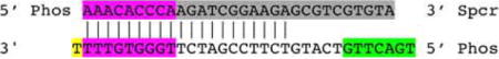
Because the DPM tag will ligate to both ends of the double-stranded DNA molecule, we designed the DPM tag to ensure that we would only read the barcode sequence from one sequencing read (Read2), rather than both. To achieve this, we included a 3′ spacer on the top strand. This prevents the top strand of the Odd tag from ligating to genomic DNA. This modification is also critical for successful amplification of the barcoded DNA by preventing hairpin formation of the single stranded DNA during the initial PCR denaturation because otherwise both sides of the tagged DNA molecule would have complementary barcode sequences.
“Odd” and “Even” Tags
We designed two sets of tags called the “Odd” and “Even” set. Both the Odd tags and Even tags have modified 5′ phosphate groups to allow for ligation. The Even tags are designed to have a sticky end that anneals to the Odd tags, and the Odd tags are designed to contain a sticky end that anneals to the Even tags. The Odd tags are ligated in the 1st, 3rd, 5th, … rounds of the SPRITE process and the Even tags are ligated 2nd, 4th, 6th, … rounds of SPRITE. Each of the Even and Odd tags contain a unique sequence of seventeen nucleotides.
Terminal Tag
The Terminal tags contain a sticky end that ligates to the Odd tags (green), though a Terminal tag can also be designed to ligate to an Even tag. The Terminal tag only contains a modified 5′ phosphate on the top strand. The bottom strand contains a region (grey) that contains part of the Illumina read 2 sequence, which allows for priming and incorporation of the full-length barcoded Read2 Illumina adaptor. The terminal tag contains a unique sequence of nine nucleotides (bold).
![]()
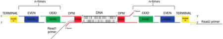
Final DNA structure
After SPRITE, the genomic DNA contains a DPM tag ligated on both ends as well as the Odd, Even, and Terminal tags. We call the full tag sequence a barcode. The product is represented below:
RNA Barcoding
For RNA tagging, we use the same approach as above, except the first ligation to the RNA is an RNA Phosphate Modified (RPM) tag. The RPM tag is designed with a ssRNA overhang to specifically ligate RNA molecules using a single-stranded RNA ligase. This RNA-specific ligation tags RNA molecules in order to distinguish a molecule as RNA, rather than DNA, on the sequencer. The RPM tag contains a distinct sequence relative to DPM (pink region) and serves as a RNA-specific tag to mark each read as RNA. However, the sticky end is identical to that contained on the DPM tag (green sequence) to enable barcoding of both DNA and RNA simultaneously. The bottom strand of the RPM tag (TGACTTGCTGACGCTAAGTCCATCCTATCTACATCCG) is phosphorylated after ligation of the RPM tag to RNA to ensure that the RPM tags do not form chimeras and ligate to each other during the ssRNA ligation of the RPM tag. The 3′ spacer on the top strand (/5Phos/rArUrCrArGrCrArCrCrCrGrGATGTAGATAGGATGGACTTAGCGTCAG/3SpC3/) of the RPM tag prevents ligation of single-stranded RPM molecules and from forming chimeras during ligation.
![]()
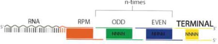
Final RNA structure
The final RNA product after SPRITE contains the RPM, Odd, Even, and Terminal tags. We call the full tag sequence a barcode. The product is represented below:
cDNA tag
In order to amplify cDNA molecules, we ligate a cDNA tag to the 3′end of all cDNA molecules. The cDNA tag contains a five-nucleotide sequence that identifies the tagged molecule as RNA in read 1 during sequencing (blue). The cDNA tag also contains a sequence that is part of the Illumina Read 1 primer (green). It is 5′phosphate modified to ligate to the 3′end of cDNA, and contains a 3′spacer to prevent chimeras of tags.
![]()
Final Library Amplification Primers
DNA and RNA libraries are amplified using common primers that incorporate the full Illumia sequencing adaptors. These are the Read 1 primer (AATGATACGGCGACCACCGAGATCTACACTCTTTCCCTACACGACGCTCTTCCGATC T) and the Read 2 primer (CAAGCAGAAGACGGCATACGAGATGCCTAGCCGTGACTGGAGTTCAGACGTGTGCT CTTCCGATCT). The Read 1 primer amplifies the top strand of the DPM tag on DNA and cDNA tag on RNA, and adds the Illumina Read 1 sequence to each molecule. The Read 2 primer amplifies the terminal tag on both DNA and cDNA, and adds the Illumina Read 2 sequence to the molecule.
SPRITE Data Processing, Cluster Generation, and Heatmap Generation
All SPRITE data was generated using Illumina paired-end sequencing on the HiSeq 2500 or NextSeq 500. Read pairs were generated with at least 115 x 100 bps. The reads have the following structure: Read 1 contains genomic DNA positional information and the DPM or cDNA tag, and Read 2 has the remaining tags. See Table S6A for number of human and mouse reads during all steps of filtering prior to cluster generation.
Barcode identification
SPRITE barcodes were identified by parsing the first DNA tag sequence from the beginning of Read 1 and the remainder of the tags were parsed from Read 2. We identified these tag sequences using a hashtable populated with the known sets of DPM, Odd, Even, and Terminal tags that were added to these samples. We allowed for up to two mismatches to each internal tag of the Odd and Even tags to account for possible sequencing errors. Because the tags were designed to contain at least four mismatches to any other tag sequence, this enables robust error correction. For DPM and terminal tag alignments, we did not tolerate any mismatches due to their shorter unique barcode sequences. We excluded any reads that did not contain a full set of all ligated tags (DPM, Odd, Even, Odd, Terminal) in the order expected from the experimental procedure. We also excluded all read pairs where we could not unambiguously map the barcode. We stored the barcode string to the name of each read in the FASTQ file.
Alignment to genome
We aligned each read to the appropriate reference genome (mm9 for mouse and hg19 for human) using Bowtie2 (v2.3.1) with the default parameters and with the following deviations. We trimmed the 11 base pair tag sequence (DPM) from Read 1 using the –trim5 11 parameter. To account for a short genomic fragment that might lead to additional tag sequences being included on the 3′end, we used a local alignment search (–local). The corresponding SAM file was sorted and converted to a BAM file using SAMtools v1.4. The barcode string is stored in the name of each record of the BAM file.
Repeat Masking and Filtering Low Complexity Sequences
We filtered the resulting BAM file for low quality reads, multimappers, and repetitive sequences. First, we removed all alignments with a MAPQ score less than 10 or 30 (heatmaps were generated for both). Second, we removed all reads that had >2 mismatches to the reference genome. Third, we removed all alignments that overlapped a region that was masked by Repeatmasker (UCSC, milliDiv < 140) using bedtools (v2.26.0). Fourth, we removed any read that aligned to a non-unique region of the genome by excluding alignments mapping to regions generated by the ComputeGenomeMask program in the GATK package (readLength=35nt mask). In the human maps, all reads that overlap with an annotated HIST gene were removed for analysis of the histone locus in Figure 2.
Identifying SPRITE clusters
To define SPRITE clusters, all reads that have the same barcode sequence were grouped into a single cluster. To remove possible PCR duplicates, all reads starting at the same genomic position with identical barcodes were removed. We generated a SPRITE cluster file for all subsequent analyses where each cluster occupies one line of the resulting text file containing the barcode name and genomic alignments.
Visualizing SPRITE clusters
Multi-way interactions were identified by counting how often multiple genomic regions simultaneously interact in individual SPRITE clusters. In Figures 2, S2, 4, and 5, rows show individual SPRITE clusters there multiple regions simultaneously interact and black lines denote genomic bins (typically 1Mb or 25kb) with at least one read within these clusters.
RNA-DNA SPRITE analysis
RNA and DNA sequences were separated by the presence of a cDNA tag or DPM tag in the first 9 nucleotides of the Read 1 sequence, respectively. RNA-tagged reads, identified by the cDNA tag, were aligned to ribosomal RNA sequences (28S, 18S, 5S. 5.8S, 4.5S, 45S) as well as other RNAs of interest such as snoRNAs, snRNAs including spliceosomal RNAs, and Malat1. Any RNA sequences that did not align to this set of RNA genes of interest were aligned to the mm9 genome using bowtie2. DNA-tagged sequences, containing the DPM tag, were aligned to mm9. All RNA and DNA reads were subsequently filtered by edit distance and MAPQ score as described above; DNA reads were additionally filtered with a DNA mask file. See Table S6B for number reads during all steps of filtering prior to cluster generation.
Generating pairwise contacts and heatmaps from SPRITE Data
To compute the pairwise contact frequency between genomic bins i and j, we counted the number of SPRITE clusters that contained reads overlapping both bins. Specifically, we counted the number of unique SPRITE clusters overlapping the two bins and not the number of reads contained within them. In this way, if a SPRITE cluster contains multiple reads that mapped to the same genomic bin, we only count the SPRITE cluster once to eliminate possible PCR duplicates. Because the number of pairwise contacts scales quadratically based on the number of reads (n) contained within a SPRITE cluster, larger clusters will contribute a disproportionally large number of the contacts observed between any two bins. To account for this, we reasoned that a minimally connected graph containing n reads would contain n-1 contacts. Therefore, we down-weighted each of the n(n-1)/2 pairwise contacts in a SPRITE cluster such that each pairwise contact has a weight of 2/n. In this way, the total contribution of pairwise contacts from a cluster is proportional to the minimally connected edges in the graph. This also ensures that the number of pairwise contacts contributed by a cluster is linearly proportional to the number of reads within a cluster.
Pairwise contacts were computed using multiple different bin sizes (10kb, 20kb, 25kb, 40kb, 50kb, 200kb, 250kb, 1Mb) to generate contact maps at different genomic resolutions. SPRITE contact maps were normalized by read coverage using Hi-Corrector (Li et al., 2015). Contacts occurring within the same bin (i.e. along the diagonal, i=j) were not considered to avoid any chance of possible PCR duplicates generating false-positive interactions. All low coverage bins are masked in heatmaps.
SPRITE processing details and scripts for performing this processing are available at: https://github.com/GuttmanLab/sprite-pipeline/wiki
Human-mouse mixing experiment
Human HEK293T cells and mouse pSM33 cells were crosslinked, lysed, and DNAse digested separately. The two lysates were then combined at equimolar concentration and coupled to NHS beads at a ratio of 620, 125, 60, 25, 6, 1.2, 0.5, 0.25, 0.125 molecules per NHS bead. Reads were aligned to both hg19 and mm9. All reads aligning to both species were removed, and species-specific reads were used to determine the amount of inter-species contacts and normalized by the expected number of contacts. For the experiments in the paper, we selected a coupling efficiency of 0.125 to 0.25 molecules/bead because it provided a small number of spurious contacts while minimizing the number of beads used in the experiment.
Comparison of SPRITE and Hi-C data
Hi-C contact maps for mouse embryonic stem cells (Dixon et al., 2012) and human GM12878 cells (Rao et al., 2014) were normalized by read coverage using Hi-Corrector (Li et al., 2015).
Compartments
We identified A and B compartments and insulation scores for SPRITE and Hi-C using cworld (Dekker lab, https://github.com/dekkerlab/cworld-dekker). To calculate compartment eigenvectors, we used the cworld script “matrix2compartment.pl” with default parameters with contact maps binned at 1Mb resolution as input. For human chromosomes, compartment eigenvectors were calculated separately for each chromosome arm. Bias in coverage of reads towards the A compartment was calculated as the observed percentage of total reads that aligned to regions in the A compartment divided by the expected percentage of total A compartment reads assuming a uniform distribution of read coverage. We note that differences in distance decay profiles between different cluster sizes, such as those observed in Figure 3B-C, occur despite comparable genomic coverage in both the SPRITE and Hi-C data (Table S2A).
TADs
To calculate insulation scores, we used the cworld script “matrix2insulation.pl”. For human insulation scores, we used the parameters “–ss 100000 –im iqrMean –is 600000 –ids 400000” with contact maps binned at 50kb resolution. For mouse insulation scores, we used the parameters “–ss 80000 –im iqrMean –is 480000 –ids 320000” with contact maps binned at 40kb resolution.
Loops
We performed aggregate peak analysis (APA) on mouse and human contact maps in both HiC and SPRITE data binned at 10kb resolution as previously described (Rao et al., 2014). Positions for loops with end points separated by at least 200kb were obtained from mouse CH12-LX cells (1493 loops) and human GM12878 cells (5789 loops) (Rao et al., 2014). Aggregate contact maps were computed for the median contact frequency in regions +/− 200kb of the loops.
Analysis of higher-order k-mer interactions
We enumerated all higher-order k-mers represented in the SPRITE data at 1 megabase (Mb) resolution. We retained k-mers that were observed in at least 5 independent SPRITE clusters. We found that the greatest determinant of k-mer frequency, similar to pairwise frequency, was linear genomic distance. Accordingly, to assess the significance of a given k-mer, we compared the observed frequency of a given k-mer to the expected frequency of other k-mers containing the same genomic distance at different positions across the genome (Figure S2A). See “Determining significant higher-order k-mer interactions” below for further details on how significance was computed for each k-mer.
SPRITE Cluster Size: Comparison of SPRITE contacts in different cluster sizes
An individual SPRITE cluster is defined as a set of reads that all contain the same barcode sequence. Accordingly, the size of a SPRITE cluster is defined as the number of reads that have the same barcode sequence. We separated SPRITE clusters into four groups: clusters with 2 to 10 reads, 11 to 100 reads, 101 to 1000 reads, and clusters with 1001 or more reads. Contact maps were generated separately for each group of clusters as described above but without down-weighting for cluster size. We analyzed the relationship between genomic distance and contact frequency by computing the average contact frequency between bins separated by 40kb, 80kb, 120kb and so forth up to 100Mb. To compare heatmaps across different cluster sizes, we normalized contact frequencies by the maximum observed value such that overall contact frequency ranges from 0 to 1 for each cluster size. To examine A compartment interactions in different cluster sizes, we calculated the average contact frequency between all 1Mb bins on mouse chromosome 2 and the bins within a 9Mb A compartment region (25 to 34Mb) and normalized these values to range from 0 to 1 for each cluster size. These contact frequencies were down-weighted by cluster size (as described above).
Additionally, we compared each SPRITE cluster size group according to the percent of contacts that occurred between two regions in the same TAD, regions in the same compartment (A or B), or regions on the same chromosome. Two regions were considered to be in the same “local” or “contiguous” compartment only if no compartment switches occurred in the linear genomic span between them. Two regions were considered to be in the same “non-local” or “discontiguous” compartment if compartment switches exist between them, but they are nevertheless both in A compartment regions or both in B compartment regions.
Defining the “active” and “inactive” inter-chromosomal DNA hubs
Hub definitions
The two “active” and “inactive” inter-chromosomal hubs were identified solely based on DNA contacts. Specifically, we identified significant inter-chromosomal interactions occurring between all 1Mb genomic regions (see below). These significant contacts cluster into 2 “sets” of DNA regions, such that there is a large degree of interconnectivity among genomic regions within set 1 and among regions within set 2. There is no connectivity between regions in set 1 and regions in set 2. Because of these two properties, we defined these sets of interactions as two distinct “hubs” of inter-chromosomal contacts. However, once these hubs were identified based solely on DNA contact frequencies, we investigated what features are associated with the DNA regions contained within each hub (see below). Specifically, we noticed that genomic regions in one of the hubs is primarily gene-poor and depleted of RNA PolII signal. In contrast, genomic regions in the other hub were highly gene-dense and contained high levels of RNA PolII occupancy. Based on these properties, we simply referred to these hubs as the “inactive hub” and “active hub” respectively.
Analysis of inter-chromosomal interactions
To identify significant inter-chromosomal interactions, we removed all intra-chromosomal contacts from the ICE normalized inter-chromosomal heatmap. We then calculated an interaction p-value using a one-tailed binomial test where the expected frequency assumes a uniform distribution of inter-chromosomal contacts. We used contact maps binned at 1Mb resolution based on SPRITE clusters containing 2 to 1000 reads without down-weighting for cluster size. We built a graph where nodes represent a 1Mb bin and edges represent connections between 2 bins. We filtered edges to reduce potentially spurious contacts that may be caused by outlier bins by looking for consistency of contacts across at least 3 consecutive bins. Specifically, we only included an edge between two bins (i and j) when the edge connecting i and j was significant and all interacting pairs i±1 and j±1 were also significant. This approach produced two networks of inter-chromosomal interactions that were defined as the inactive hub (nucleolar hub, p-values ≤ 10−10) and active hub (active hub, p-values ≤ 10−8).
Identifying features associated with each hub
To identify features that distinguish these hubs and the rest of the genome, we calculated various properties, such as average gene density and average number of Pol II ChIP-seq peaks for each genomic region in these hubs and compared these to a set of control regions not contained in either hub, but with the same distribution of lengths. In Figure 3F, gene density is calculated as the number of genes per 1Mb region and Pol II occupancy is calculated as number of ChIP-seq peaks per 1Mb region (ENCODE). The properties we analyzed included the following: gene density, number of enhancers (Whyte et al., 2013), number of super-enhancers (Whyte et al., 2013), histone modifications (H3K27ac, H3K4me1, H3K36me3, H3K4me3), GRO-seq signal (Jonkers et al., 2014), number of Pol II ChIP-seq peaks, number of DNase-seq peaks. Histone modification, Pol II ChIP-seq and DNase-seq data were obtained from ENCODE. Because one of the two hubs was highly enriched in active chromatin marks, RNA PolII, and GRO-seq signal we defined it as the “active hub”, while the other was depleted for these features of high transcriptional activity and was therefore defined as the “inactive hub”.
SPRITE contact frequency with the nucleolar and active hubs
We defined contact frequency with the nucleolar and active hubs for each 1Mb bin based on the average inter-chromosomal contact frequency with all regions in the nucleolar and active hub, respectively. p-values were calculated for these contact frequencies using a one-tailed binomial test where the expected frequency assumed a uniform distribution of inter-chromosomal contacts and are shown in units of –log10(p-value) in the corresponding figures. Contact frequencies with these hubs were compared to RNA localization (described above) and data from ChIP-seq (e.g., Pol II, H3K4me3) and GRO-seq experiments obtained from ENCODE and from (Jonkers et al., 2014), respectively.
Analysis of inter-chromosomal centromere interactions
Mouse inter-chromosomal centromere interactions were defined as interactions between the closest bin to the centromere that can be mapped (“peri-centromeric bin”, usually 3-4Mb) and any given region on a different chromosome. To analyze these interactions, we calculated the median contact frequency between the peri-centromeric bin of each mouse chromosome and bins on different chromosomes at specific distances ranging from 1Mb to 100Mb. We then computed the mean contact frequency for each centromere distance across all mouse chromosomes. We excluded chromosomes 14 and X from this analysis because they do not have reads that uniquely map within 4Mb of the centromere.
Analysis of lamina associated domain interactions
Lamina associated domains (LADs) were obtained from Peric-Hupkes et al., 2010 (Peric-Hupkes et al., 2010). We calculated a genome-wide LAD interaction heatmap by summing the number of contacts between all pairs of LADs and normalizing by read coverage using Hi-Corrector (Li et al., 2015). To compare the frequency of LAD/LAD contacts with LAD/non-LAD in SPRITE with Hi-C, we classified each 1Mb bin as “LAD” or “non-LAD” based on whether or it had a Lamin B1-DamID score above the median. We then computed the median contact frequency between bins separated by specific distances ranging from 1Mb to 80Mb for pairs of bins classified as LAD/LAD and LAD/non-LAD.
Defining genomic regions near ribosomal DNA clusters
The precise location of ribosomal DNA genes in both mouse and human are unknown because they are not mapped in the reference genomes. However, approximate locations have been reported based on non-sequencing methods. In mouse, rDNA genes are encoded from the centromere-proximal regions of chromosomes 12, 15, 16, 18, and 19 (Suzuki et al., 1990). In human, rDNA genes are encoded on chromosomes 13, 14, 15, 21 and 22 (Németh et al., 2010; Pederson, 2011). Importantly, the locations of rDNA genes can be strain-dependent in mice (Strongin et al., 2014; Suzuki et al., 1990). For instance, on chromosome 15, the 129 allele of the F1-21 hybrid mouse line does not include rDNA genes, while it does on the Cast allele (Strongin et al., 2014). This hybrid line was used for all DNA-DNA mapping methods and nucleolar hub identification. Instead, we performed our rRNA-DNA maps in another mouse cell line (pSM33), which is derived from a C57BL/7 x 129SV mouse, which are reported to contain rDNA genes on both alleles of chromosome 15. This difference in the rDNA locations between strains may explain why we observe a stronger enrichment of rRNA on chromosome 15 in the rRNA-DNA maps than in the DNA nucleolar hub contact maps (Figure 4A).
Ribosomal RNA (rRNA) localization quantification
To quantify the localization of ribosomal RNA (rRNA) across the genome, we split SPRITE clusters into two groups, one with clusters that contained at least 1 rRNA read (rRNA positive clusters) and the other with clusters lacking any rRNA reads (rRNA negative clusters). We then calculated the ratio of rRNA positive clusters to rRNA negative clusters for each 1Mb bin, normalizing for total number of clusters in each group, and defined this ratio as the rRNA enrichment for each bin. We calculated rRNA enrichment p-values for each bin using a one-tailed binomial test where the expected frequency was based on the rRNA negative clusters and are shown in units of –log10(p-value) in Figure 4A. To quantify Malat1 and U1 localization, we obtained Malat1 and U1 RAP-DNA alignments from Engreitz et al.(Engreitz et al., 2014) and calculated Malat1 and U1 enrichment for each 1Mb bin by normalizing to input RAP-DNA alignments.
Measurement of Distance between DNA Loci and Nuclear Bodies using microscopy (Histochoice Fixation)
DNA-FISH Combined with Immunofluorescence
DNA fluorescence in situ hybridization (DNA-FISH) was performed with Agilent SureFISH DNA-FISH probes following the manufacturer’s protocol with adaptations noted below. Probe sets used for FISH were designed by Agilent technologies using their standard procedures against genomic regions defined in Table S6C. Female F1-21 cells were cultured on Poly-D Lysine (Sigma Aldrich) and gelatin (Sigma Aldrich) coated coverslips. The coverslips were fixed using 300uL of Histochoice for 10 minutes at room temperature, then dehydrated through incubation in a series of graded ethanol concentrations up to 100% ethanol, and air-dried. The coverslips were then turned cell-side down onto a 5uL mixture of a custom probe set targeting a selected DNA locus (Agilent) and SureFISH Hybridization Buffer (Agilent, G9400A). The coverslips and probe mixture were denatured for 8 minutes at 83°C, then incubated at 37°C overnight in a humidified chamber. The following morning, coverslips were washed with FISH Wash Buffer 1 (Agilent, G9401A) at 73°C for 2 min on a shaking incubator at 300 rpm, and FISH Wash Buffer 2 (Agilent, G9402A) at room temperature for 1 minute. Coverslips were then rehydrated and suspended in 1X PBS in preparation for immunofluorescence staining.
Following DNA-FISH probe hybridization, immunofluorescence was performed. Coverslips were permeabilized with 0.1% Triton-X in PBS at room temperature for 10 minutes, then blocked with 1X blocking buffer (Abcam ab126587) in PBS at room temperature for one hour. The coverslips were then incubated with primary antibodies in a humidified chamber at room temperature for one hour for anti-Nucleolin or overnight at 4°C for anti-SC35. The coverslips were washed with 0.1% Triton-X in PBS at room temperature, then incubated with secondary antibodies in a humidified chamber at room temperature for one hour. Coverslips were washed with PBS and H2O and mounted on slides in ProLong® Gold antifade reagent with DAPI (Life Technologies, P36931). The primary antibodies used for IF were rabbit polyclonal anti-Nucleolin (Abcam; ab22758; 1:1000) and mouse monoclonal anti-SC35 (Abcam; ab11826; 1:200). The secondary antibodies used for IF were Alexa Fluor® 647 goat anti-rabbit IgG (H+L) (Thermo Fisher Scientific; A21244; 1:300) and DyLight® 650 goat anti-mouse IgG (H+L) (Bethyl; A90-116D5; 1:300).
Microscopic imaging
DNA FISH/IF samples were imaged using a Leica DMI 6000 Deconvolution Microscope, with a z-stack collected for each channel (4 μm; step size, 0.2 μm). The objectives used were the Leica HC PL APO 63x/1.30 GLYC CORR CS2 objective and the Leica HCX PL APO 100X/1.40- 0.70na OIL objective. Samples were also imaged with a ZEISS Laser Scanning Microscope (LSM) 800 with the ZEISS i Plan-Apochromat 63x/1.4 Oil DIC M27 objective, with a z-stack collected for each channel (step size, 0.37 μm). Deconvolution was performed using Huygens Professional version 17.04 (Scientific Volume Imaging, The Netherlands, software available at http://svi.nl) using the built-in theoretical point spread function, the classic maximum likelihood estimation (CMLE) algorithm, a signal to noise ratio of 20, and 50 iterations.
Calculating distance between DNA loci
The nuclei of individual cells were identified by DAPI staining, and cells containing two spots per DNA-FISH channel were identified manually. Images were cropped to only contain the identified cell. Analysis of cells in three dimensions was performed using Imaris version 8.4.1 (Bitplane Inc, software available at http://bitplane.com) with the ImarisXT module. Both alleles for each DNA locus were defined by applying the Imaris “Spot” function (diameter = 0.5μm, background subtraction) on the corresponding fluorescent channel. The distance between DNA loci was calculated by running the XTension “Distances Spots to Surfaces” function and manually recording the smallest distance between alleles of differing loci.
Calculating distance between DNA loci and nuclear bodies
The nucleolus and nuclear speckle, identified by immunofluorescence of nucleolin and SC35 respectively, were defined in Imaris by performing the Imaris “Surface” function (detail = 0.126 μm, absolute intensity). Custom Imaris XTensions were used to calculate a distance transform approximating Euclidean distance for the region outside of the generated surface (“Batch Process Function” by Pierre Pouchin and “Distance Transformation Outside Object For Batch” by Matthew Gastinger, obtained on open.bitplane.com). The edges of the surface served as boundary voxels; regions inside the surface were assigned a distance transform value of 0. The distance of an allele to the nucleolus or nuclear speckle was defined as the minimum distance transform value of the corresponding spot, from the edge of the surface to the nearest edge of the DNA-FISH sphere.
Measurement of Distance between DNA Loci and Nuclear Speckles using microscopy (Formaldehyde Fixation)
Immunofluorescence
Immunofluorescence was performed followed by non-barcoded DNA sequential FISH (DNA seqFISH) (Takei et al., 2017) with modified steps. Female F1-21 cells were cultured and fixed on Poly-D Lysine (Sigma Aldrich) and human laminin (BioLamina LN511) coated coverslips (Thermo Scientific Gold Seal 3421) using 4% Formaldehyde (Pierce) for 10 minutes at room temperature, washed with 1X PBS, and stored in 70% ethanol for more than overnight at −20°C. The coverslips were air dried, incubated with 0.2 μm blue fluorescent (365/415) beads (Thermo Scientific F8805) with 2000-fold dilution in 2X SSC at room temperature for 5 minutes for the alignment of images. The coverslips were then washed twice with 2X SSC, and blocked with Blocking Buffer (5% BSA GEMINI 700-106P, 1X PBS and 0.3% Triton-X) at room temperature for 30 minutes. The coverslips were washed with 0.3% Triton-X in 1X PBS at room temperature, and incubated with a primary antibody of mouse monoclonal anti-SC35 (Abcam; ab11826; 1:200) in Antibody Dilution Buffer (1% BSA, 1X PBS and 0.3% Triton-X) at 4°C overnight. The coverslips were then washed with 0.3% Triton-X in 1X PBS at room temperature, and incubated with secondary antibody DyLight® 488 goat anti-mouse IgG (H+L) (Bethyl; A90-116D2; 1:300) in Antibody Dilution Buffer at room temperature for 1 hour. Coverslips were washed with 1xPBS, incubated with DAPI and imaged in Anti-Bleaching Buffer (50 mM Tris-HCl pH 8.0, 300 mM NaCl, 2X SSC, 3 mM Trolox [Sigma 238813], 0.8% D-glucose, 100-fold diluted Catalase [Sigma C3155] and 0.5 mg/mL Glucose oxidase [Sigma G2133]). Imaging conditions are described below under “Microscopic Imaging.”
DNA seqFISH
Following the immunofluorescence, non-barcoded DNA seqFISH experiments were performed on the same coverslips. Single-stranded DNA FISH probes were designed against specific mouse regions defined in Table S6D, purchased as an oligoarray pool (Twist Bioscience), and generated with limited cycle PCR, in vitro transcription, reverse transcription as described previously (Takei et al., 2017). After immunofluorescence imaging, the coverslips were washed with 1X PBS twice at room temperature, and incubated with 0.1 mg/mL RNaseA (Thermo Scientific) at 37°C for 1 hour. The coverslips were washed and dried with 1x PBS, 70% ethanol and 100% ethanol. The coverslips were then heated at 90°C for 10 minutes with 50% formamide in 2X SSC. The coverslips were then hybridized with the probe pool at 37°C overnight in 50% formamide, 2X SSC and 0.1 g/mL dextran sulfate (Sigma-Aldrich D8906). After incubation with the primary probe pool, the coverslips were washed with 55% Wash Buffer (55% formamide, 0.1% Triton-X, 2X SSC) at room temperature for 30 minutes, and hybridized with readout probes that were 15-nucleotides in length (IDT), which can bind to the readout sequences on the primary probes, coupled to Alexa Fluor 647 (Lifetech) or Cy3B (GE Healthcare) at 50 nM final concentration at room temperature for 20 minutes in 10% EC Buffer (10% ethylene carbonate [Sigma Aldrich E26258], 2X SSC and 0.1 g/mL dextran sulfate [Sigma-Aldrich D4911]). The coverslips were then washed with 10% Wash Buffer (10% formamide, 0.1% Triton-X and 2X SSC) at room temperature for 5 minutes, stained with DAPI and imaged in Anti-Bleaching Buffer. Imaging conditions are described below under “Microscopic Imaging.” Following the imaging, the coverslips were washed with 2X SSC once at room temperature, incubated in 55% Wash Buffer at room temperature for 5 minutes for readout probe displacement, and then washed three times with 2X SSC. To check the readout probe displacement, the coverslips were imaged with all imaging channels in Anti-Bleaching Buffer. The coverslips were then re-hybridized with another set of readout probes at 50 nM final concentration at room temperature for 20 minutes in 10% EC Buffer, stained with DAPI and imaged in Anti-Bleaching Buffer. In total, three rounds of hybridizations with two colors were carried out for DNA-seqFISH to image six regions.
Microscopic Imaging
Samples were imaged with a microscope (Leica DMi8 automated) equipped with a confocal scanner unit (Yokogawa CSU-W1), a sCMOS camera (Andor Zyla 4.2 PLUS), 63X oil objective lens (Leica NA 1.40), and a motorized stage (ASI MS2000). Lasers from CNI and filter sets from Semrock were used. Images were acquired with 0.35 μm z steps.
Calculating distance between DNA loci and nuclear bodies
Image processing was carried out using ImageJ and MATLAB. Images between different imaging rounds were registered and aligned using 405 nm channel images, which contain DAPI and 0.2 μm blue fluorescent beads signals, with MATLAB’s imregtform and imwarp functions. To remove the effects of chromatic aberration, 0.1 μm TetraSpeck beads (Thermo Scientific T7279) were used to create geometric transforms to align different fluorescence channels. Cells with two DNA-FISH spots for a given DNA loci were visually identified and confirmed. Nuclei of individual cells were identified by DAPI staining, and the precise location of DNA-FISH spots were defined as described previously (Takei et al., 2017). The nuclear speckles identified by immunofluorescence of SC35 were defined using ImageJ’s rolling ball background subtraction algorithm with a radius of 3 pixels, followed by ImageJ’s auto threshold algorithm. The distance of an allele to the nuclear speckle was defined as the minimum distance of a DNA-FISH spot to the boundary of any nuclear speckle in the corresponding cell.
Technical challenges associated with quantitatively measuring multi-way interactions using seqFISH
There are significant technical challenges that precludes us from quantitatively measuring the co-occurrence of multiple DNA sites around a nuclear body across many individual cells by microscopy. Specifically, following computational and manual image processing, approximately 10-15% of all cells imaged have DNA FISH signal identified for a single DNA region of interest. Accordingly, the percentage of cells that contain FISH signals for two DNA regions in the same cell is approximately 1-2%. This is further compounded when increasing to 3-way interactions in the same cell (0.1-0.3% of cells). Specifically, to identify 2 examples where two distinct DNA regions organize around the same nuclear speckle required imaging and analysis of ~800 individual cells. 15 (of ~800) individual cells contained FISH signals for two active hub DNA regions in the same cell. 2 (of 15) cells showed simultaneous co-association around the same speckle. In contrast, for an active hub and control DNA region, we observe 0 (of 21) cells that showed simultaneous co-association around the same speckle.
Comparison of SPRITE and DNA FISH
To compare SPRITE and DNA FISH measurements, we used SPRITE contact frequencies from contact maps binned at 1 Mb resolution based on SPRITE clusters containing 2 to 1000 reads without down-weighting for cluster size. We note that similarly high correlations between SPRITE and DNA FISH measurements were observed when large SPRITE clusters (>100 reads) are included in the analyses (consistent with the observation of inter-chromosomal interactions in larger clusters in Figure 3D), both with and without weighting for cluster size (Table S6E). SPRITE contact frequencies were obtained for 1 Mb bins that overlapped with each DNA FISH probe region and compared to DNA FISH distance measurements with the corresponding probe region.
QUANTIFICATION AND STATISTICAL ANALYSIS
Determining significant higher-order k-mer interactions
We found that the greatest determinant of k-mer frequency, similar to pairwise frequency, was linear genomic distance. Accordingly, to assess the significance of a given k-mer, we compared the observed frequency of a given k-mer to the expected frequency of k-mers containing the same genomic distance. To do this, for a given k-mer, we computed the genomic distance separating each region in the k-mer and randomly sampled regions across the genome containing the same linear genomic distances and computed the number of SPRITE clusters containing these k-mers (Figure S2A). SPRITE cluster counts were normalized by cluster size to define a weighted score and prevent large SPRITE clusters from dominating the number of k-mer observations. For k-mers of interest, enrichment was defined as the observed weighted SPRITE counts divided by the average across 100 random permutations. Genome-wide analysis was performed across 10 random permutations to identify an initial subset of enriched k-mers. We also retained the number of permutations that had an observed frequency larger than observed for the k-mer of interest and we report this percentile to rank each higher-order k-mer.
Defining significant inter-chromosomal contacts
To identify significant inter-chromosomal interactions, we removed all intra-chromosomal contacts from the ICE normalized inter-chromosomal heatmap. We then calculated an interaction p-value using a one-tailed binomial test where the expected frequency assumes a uniform distribution of inter-chromosomal contacts. We used contact maps binned at 1Mb resolution based on SPRITE clusters containing 2 to 1000 reads without down-weighting for cluster size. We built a graph where nodes represent a 1Mb bin and edges represent connections between 2 bins. We filtered edges to reduce potentially spurious contacts that may be caused by outlier bins by looking for consistency of contacts across at least 3 consecutive bins. Specifically, we only included an edge between two bins (i and j) when the edge connecting i and j was significant and all interacting pairs i±1 and j±1 were also significant.
Plots and statistical analysis
Plots and statistics were generated in GraphPad Prism version 7.0c, MATLAB R2016a (MathWorks), R version 3.3.1 (Pearson and Spearman correlation coefficients), and Microsoft Excel v16.10. For all microscopy measurements, the exact value of the number of cells used (n) and precision measurements used (mean ± SEM) is reported in the corresponding figure legends and also in Figures S4D, S6B.
DATA AND SOFTWARE AVAILABILITY
Detailed SPRITE protocols are available at http://guttmanlab.caltech.edu/protocols.php. SPRITE software is available at https://github.com/GuttmanLab/sprite-pipeline/wiki. All datasets reported in this paper are available at the Gene Expression Omnibus with accession number GEO: GSE114242.
KEY RESOURCES TABLE
| REAGENT or RESOURCE | SOURCE | IDENTIFIER |
|---|---|---|
| Antibodies | ||
| rabbit polyclonal anti-Nucleolin | Abcam | Cat# ab22758, RRID:AB_776878 |
| mouse monoclonal anti-SC35 | Abcam | Cat# ab11826, RRID:AB_298608 |
| Alexa Fluor® 647 goat anti-rabbit IgG (H+L) | Thermo Fisher Scientific | Cat# A-21244, RRID:AB_2535812 |
| DyLight® 650 goat anti-mouse IgG (H+L) Bethyl | Cat# A90-116D5, RRID:AB_10630715 | |
| Bacterial and Virus Strains | ||
| Biological Samples | ||
| Chemicals, Peptides, and Recombinant Proteins | ||
| Disuccinimidyl glutarate (DSG) | Thermo Fisher Scientific | Cat# 20593 |
| 16% Formaldehyde (w/v), Methanol-free | Pierce | Cat# 28908 |
| Doxycycline Sigma | Cat# D9891 | |
| Critical Commercial Assays | ||
| NEBNext End Repair Module | NEB | Cat# E6050 |
| NEBNext dA-tailing Module | NEB | Cat# B6059 |
| Instant Sticky End Master Mix | NEB | Cat# M0370 |
| Deposited Data | ||
| Raw and analyzed data | This paper | GEO: GSE114242 |
| ChIP-seq (e.g., Pol II, H3K4me3, etc) in mES cells | ENCODE; https://encodeproject.org | https://www.encodeproject.org/search/?type=Experiment&assembly=mm9&biosample_type=stem+cell |
| ChIP-seq (e.g., Pol II, H3K4me3, etc) in GM12878 cells | ENCODE; https://encodeproject.org | https://www.encodeproject.org/search/?type=Experiment&assembly=hg19&biosample_term_name=GM12878 |
| GRO-seq data in mES cells | (Jonkers et al., 2014) | GEO:GSE48895 |
| TAD Triplets identified using GAM in mES cells | (Beagrie et al., 2017) | https://media.nature.com/original/nature-assets/nature/journal/v543/n7646/extref/nature21411-s3.xlsx |
| Hi-C data in mES cells | (Dixon et al., 2012) | GEO:GSE35156 |
| Hi-C data in GM12878 cells | (Rao et al., 2014) | GEO:GSE63525 |
| Malat1 and U1 RAP-DNA in mES cells | (Engreitz et al., 2014) | GEO:GSE55914 |
| Mouse ES cell super-enhancers | (Whyte et al., 2013) | http://www.cell.com/cms/attachment/2031389007/2048455341/mmc1.zip |
| Mouse ES cell enhancers | (Whyte et al., 2013) | http://www.cell.com/cms/attachment/2031389007/2048455344/mmc2.xls |
| Lamin Associated Domains in mES cells | (Peric-Hupkes et al., 2010) | https://ars.els-cdn.com/content/image/1-s2.0-S1097276510003217-mmc2.xls |
| Experimental Models: Cell Lines | ||
| F1 2-1 hybrid wild-type mouse ES cell line (129 x cast) | Kathrin Plath | (Engreitz et al., 2013) |
| pSM33 mES cell line | Kathrin Plath | (Engreitz et al., 2013) |
| GM12878 Human Lymphoblasts | Coriell Cell Repositories | GM12878, RRID:CVCL_7526 |
| Human HEK293T | ATCC | Cat# CRL-3216, RRID:CVCL_0063 |
| Experimental Models: Organisms/Strains | ||
| Oligonucleotides | ||
| SPRITE oligos and adaptors | This paper | See Table S5 |
| Recombinant DNA | ||
| Software and Algorithms | ||
| Bowtie2 (v2.3.1) | Langmead Laboratory | http://bowtie-bio.sourceforge.net/bowtie2/index.shtml |
| ComputeGenomeMask | GATK package | https://gatkforums.broadinstitute.org/gatk/discussion/1499/computegenomemask |
| Bedtools (v2.26.0) | Quinlan Laboratory | http://bedtools.readthedocs.io/en/latest/ |
| Imaris (8.4.1) | Bitplane Inc. | http://bitplane.com |
| Hi-Corrector Zhou | Laboratory | http://zhoulab.usc.edu/Hi-Corrector/ |
| Cworld Dekker | Laboratory | https://github.com/dekkerlab/cworld-dekker |
| SPRITE computational pipeline | This study | https://github.com/GuttmanLab/sprite-pipeline/wiki |
| GraphPad Prism 7 | GraphPad Software | https://www.graphpad.com/scientific-software/prism/ |
| R Software Package 3.3.1 | The R Foundation | https://www.r-project.org/ |
| Other | ||
| Resources related to the SPRITE protocol | This paper | http://www.lncrna.caltech.edu/protocols.php |
| Branson needle-tip sonicator (3 mm diameter (1/8″ Doublestep tip) | Branson Ultrasonics | Cat# 101-148-063 |
Supplementary Material
Figure S1. SPRITE accurately recapitulates genome structure measured by Hi-C, Related to Figure 1. (A) Estimate of the frequency of spurious contacts that are identified within individual SPRITE clusters. Noise was estimated by coupling crosslinked lysate from mouse ES cells and human HEK293T cells to NHS beads. The ratio of material per bead was coupled at different amounts (x-axis) and the percentage of clusters and pairwise contacts containing human and mouse reads were computed (interspecies contacts, y-axis). The red point indicates the molecule-to-bead ratio used for the SPRITE experiments in this paper. (B) Distribution of reads containing 0, 1, 2, 3, 4, 5 tags for mouse (left) and human (right) experiments. The estimate for ligation efficiency each round is determined by taking the 5th root of the fraction of reads with all 5 tags. (C) Distribution of SPRITE cluster sizes for mouse (left) and human (right) experiments. The percentage of reads was calculated for different SPRITE cluster sizes (1, 2-10, 11-100, 101-100 and over 1001) and reported as the percentage of total reads. Cluster size is defined as the number of reads with the same barcode. (D-L) SPRITE in mouse embryonic stem (ES) cells and human GM12878 lymphoblast cells was compared to Hi-C data generated in Dixon et al.(Dixon et al., 2012) and Rao et al.(Rao et al., 2014), respectively. (D) Compartment eigenvector for mouse chromosome 2 calculated using SPRITE (black) and Hi-C (red) contact maps from mouse ES cells binned at 1Mb resolution. Positive and negative values correspond to the A and B compartments, respectively. (E) Genome-wide correlation between compartment eigenvectors calculated using SPRITE (y-axis) and Hi-C (x-axis) contact maps from mouse ES cells binned at 1Mb resolution. (F) Genome-wide correlation between compartment eigenvectors calculated using SPRITE (y-axis) and Hi-C (x-axis) contact maps from human GM12878 cells binned at 1Mb resolution. (G) Insulation score profile for a region on mouse chromosome 2 (shown in Figure 1D) calculated using SPRITE (black) and Hi-C (red) contact maps from mouse ES cells binned at 40kb resolution. Local minima correspond to boundary regions. (H) Genome-wide correlation between insulation scores calculated using SPRITE (y-axis) and Hi-C (x-axis) contact maps from mouse ES cells binned at 40kb. (I) Genome-wide correlation between insulation scores calculated using SPRITE (y-axis) and Hi-C (x-axis) contact maps from human GM12878 cells binned at 40kb. (J) Examples of SPRITE and Hi-C contact maps binned at 20kb resolution (top) and 10kb resolution (bottom) showing chromatin loop interactions. CTCF ChIP-seq peaks are shown according to their positive (red) or negative (blue) motif orientation. (K) Aggregate peak analysis heatmaps for Hi-C (top) and SPRITE (bottom) in mouse ES cells binned at 10kb resolution. 1493 loops obtained from Rao et al.(Rao et al., 2014) were used in this analysis. Heatmaps show the median contact map values for each pair of 10kb bins in regions +/- 200kb of the loops. (L) Aggregate peak analysis heatmaps for Hi-C (top) and SPRITE (bottom) in human GM12878 cells binned at 10kb resolution. 5789 loops obtained from Rao et al.(Rao et al., 2014) were used in this analysis. Heatmaps show the median contact map values for each pair of 10kb bins in regions +/- 200kb of the loops.
Figure S2. SPRITE measures higher-order interactions across known genome structures, Related to Figure 2. (A) Cartoon representation of the method for identifying enriched higher-order k-mer frequencies. Given an observed k-mer, we randomly permute k-mers by randomizing the location of the genomic positions within the k-mer while preserving the spacing between its reads. The observed frequency is then normalized by the expected frequency derived from the randomly permuted k-mers. See Methods for further details. (B) Statistics of the size distribution observed in all enumerated (left) and enriched (right) k-mers in mES cells at 1Mb resolution. Enriched k-kmers are defined as those that are observed in at least 5 independent SPRITE clusters, occur >4-fold more frequently than the average of the permuted k-mers, and are observed at a frequency that is more than 90% of the permuted structures. (C) Example SPRITE clusters spanning four A compartment regions on mouse chromosome 2. The compartment eigenvector showing A (red) and B (blue) compartments is shown on top. Rows correspond to individual SPRITE clusters and colored lines denote 1Mb bins with at least 1 read. Each colored group represents a different combination of four A compartment regions interacting across several SPRITE clusters (max cluster size n=20 1Mb bins). Red shaded area demarcates the A compartment regions. Enrichments compared to randomly permuted k-mers spanning 4 or more A compartment regions in mES cells are listed in Table S1C. (D) Four examples of 3-way interactions between 3 loop anchors in human GM12878 cells. SPRITE contact maps are shown at 25kb resolution above the individual SPRITE clusters that contain all three loop anchors (max cluster size n=100 25kb bins) (E) Examples of enriched SPRITE clusters corresponding to super-enhancer TAD triplets previously identified using GAM in mES cells(Beagrie et al., 2017) (max cluster size n=100 1Mb bins).
Figure S3. SPRITE identifies long-range intra-chromosomal interactions and hubs of inter-chromosomal interactions, Related to Figure 3. (A) Relationship between contact frequency as a function of linear genomic distance observed in SPRITE (blue) and Hi-C(Dixon et al., 2012) (red) for mouse ES cells. (B) Contact frequency between a specific A (red) compartment region (R1: 25-34 Mb) and all other regions on mouse chromosome 2. Pairwise contact frequencies are shown for SPRITE (blue) and Hi-C (red). Red shaded areas represent A compartment regions. (C) Comparison of Hi-C contact map (top) with SPRITE contact maps based on SPRITE clusters with 2 to 10 reads (middle) and 11 to 100 reads (bottom) in a 12Mb region on mouse chromosome 2 binned at 40kb resolution. Contact map values are shown as the fraction of total contacts. H3K27ac ChIP-seq signal (ENCODE) from mouse ES cells is shown below. (D) Different SPRITE cluster sizes capture different scales of interactions. The percentage of pairwise contacts are quantified within structures of different sizes in the nucleus—TADs, local compartment regions, and non-local compartment regions for SPRITE clusters containing 2-10 reads (yellow), 11-100 reads (green), 101-1000 reads (blue) and 1001 or more reads (purple) compared against Hi-C (red). (E) Inter-chromosomal contacts between chromosomes 12 through 19 in mES cells binned at 1Mb resolution. Interaction p-values are shown for SPRITE clusters with 1001+ reads (upper diagonal) and for SPRITE contacts that have been down-weighted by cluster size (lower diagonal). p-values were calculated based on inter-chromosomal interaction frequencies and are shown in units of -log10 (p-value). (F) Comparison of SPRITE (upper diagonal) and Hi-C (lower diagonal) inter-chromosomal contacts between chromosomes 12 through 19 in mES cells binned at 1Mb resolution. SPRITE contacts are based on clusters with 2 to 1000 reads. Values shown are the fraction of total contacts. (G) Comparison of inter-chromosomal contacts between chromosomes 12 through 19 based on SPRITE clusters with 2 to 1000 reads (upper diagonal) or 2 to 10 reads (lower diagonal) in mES cells binned at 1Mb resolution. Values shown are the fraction of total contacts. (H, K) Examples of inter-chromosomal interactions that comprise the Inactive Hub (top, blue) and Active Hub (bottom, red) in mES and GM12878 cells, respectively. Inactive and active hub regions are colored on the chromosome ideogram as blue and red, respectively. Interaction p-values were calculated using unweighted contact frequencies from SPRITE clusters with 2 to 1000 reads and are shown in units of −log10 (p-value). (I, L) Ideogram showing inactive hub (blue) and active hub (regions) on each mouse and human chromosome, respectively. Centromere regions are demarcated in grey. (J) Box plots showing the distribution of different features associated with high RNA Polymerase II transcription (DNase-seq from ENCODE, GRO-seq (Jonkers et al., 2014)), active chromatin marks (H3K27ac, H3K4m1, H3K36me3, H3K4me3 from ENCODE), and regulatory features (super-enhancers, enhancers(Whyte et al., 2013)) in mES cells. (M) Circos diagram of significant inter-chromosomal interactions in GM12878 cells. Interactions are identified from unweighted inter-chromosomal contact maps in SPRITE clusters containing 2 to 1000 reads. Interactions with p-values less than 10−8 are shown. Two distinct networks of non-interacting connections are shown in blue (inactive hub) and red (active hub). (N) Box plots showing the distribution of gene density (top) and RNA polymerase II (Pol II) occupancy (bottom) for regions in the inactive hub, nucleolar hub, or neither hub in GM12878 cells. Gene density is calculated as genes per 1Mb and Pol II occupancy is calculated as the number of ChIP-seq peaks per 1Mb (from ENCODE).
Figure S4. Genomic DNA in the inactive hub is organized around the nucleolus, Related to Figure 4. (A) A schematic of the RNA-DNA SPRITE procedure. SPRITE was adapted to simultaneously tagged RNA and DNA molecules in crosslinked complexes during each round of split-pool tagging. (B) Most reads in the RNA-DNA SPRITE maps containing an RNA-specific tag aligned to the transcribed (+) strand of ribosomal RNA, in contrast to reads containing a DNA-specific tag which uniformly aligned with either of the two strands. (C) Comparison of ribosomal RNA localization from RNA-DNA SPRITE maps (black) and average inter-chromosomal contact frequency with regions in the inactive hub (blue) binned at 1Mb resolution for mouse chromosomes 12, 18 and 19. Inactive hub regions are shown in blue at the top of each plot. (D) Cumulative distributions for the 3D distances of 8 probe regions and the most proximal nucleolus (only the distance of the nearest allele per cell is shown). Four probe regions in the inactive hub are shown in blue, green, teal, and purple. Four control probe regions not in the inactive hub are shown in black, grey, orange, and yellow. One active hub probe region is shown in red. Number of cells measured (n) is listed for each probe. (E) Example images from immunofluorescence for nucleolin (red) combined with DNA FISH for three different DNA FISH control region probes (chr18-C1, chr18-C2 and chr19-C). (F) Comparison of the frequency of co-association of two DNA regions on different chromosomes at the same nucleolus measured by DNA FISH. Percentage of cells with two regions at the same nucleolus is reported if at least one allele for six different pairs of DNA FISH probes are 0 μm from the same nucleolus (n = 50 to 64 cells). Pairs of probes with one control region and one inactive hub region are shown in grey, and pairs of two inactive hub region probes are shown in blue.
Figure S5. Genomic DNA regions in the active hub are organized around the nuclear speckles, Related to Figure 5. (A) Box plots showing the distribution of U1 RNA enrichment to genomic DNA (top) and Malat1 RNA enrichment to genomic DNA (bottom) from Engreitz et al.(Engreitz et al., 2014) for regions in the active hub, inactive hub, or neither. (B) Comparison of U1 or Malat1 RNA-DNA (black) enrichment with average inter-chromosomal contact frequency with regions in the active hub binned at 1Mb resolution for mouse chromosomes 4 (left) and 11 (middle). Genome-wide correlation plots are shown on the right. (C, D) Example images from immunofluorescence for SC35 (red) combined with DNA FISH (green) for an active hub probe region on chromosome 2 (chr2-A) in cells fixed using 4% formaldehyde and histochoice prior to DNA FISH/IF, respectively. Inset images show the region around the arrowhead. DAPI (blue) is used to demarcate the nucleus. (E, F) Cumulative distributions for the 3D distances of 6 probe regions and the most proximal speckle (only the distance of the nearest allele per cell is shown) in cells fixed using 4% formaldehyde (n = 50 to 155 cells) and histochoice (n = 41 to 90 cells) prior to DNA FISH/IF, respectively. Three probe regions in the active hub are shown in blue, red, and green. Three control probe regions not in the active hub are shown in yellow, orange, and purple. (G) Comparison of the 3D distance to the most proximal nuclear speckle for 6 different probe regions, including 3 control regions (grey/blue) and 3 active hub regions (red). Proximity to nuclear speckles is calculated for each probe region as the percent of cells with at least 1 allele within 0 μm (left) and 0.25 μm (right) of an SC35 speckle for cells crosslinked using histochoice prior to DNA FISH/IF. (H) Comparison of the percentage of cells where two probes are within a given distance (0.5 μm, 1.0 μm and 1.5 μm) for two active hub probes (red) and an active/control pair (grey) measured in cells fixed using histochoice prior to DNA FISH/IF. The large distance between the two DNA regions likely reflects the fact that the individual DNA sites are organized around nuclear speckles rather than directly contacting each other.
Figure S6. Preferential organization relative to the nucleolus and nuclear speckles shapes the overall organization of genomic DNA in the nucleus, Related to Figure 6. (A) Genome-wide comparison of average SPRITE contact frequency to regions in the nucleolar hub (y-axis) or speckle hub (x-axis). Each dot corresponds to a 1Mb bin. Regions within the A and B compartment are colored red and blue, respectively. (B) Number of cells imaged and measured for 3D distances to the nucleolus and nuclear speckle reported in Figures 6C-D and S6D. (C) A schematic representation showing the location of the various DNA FISH probes used in Figures 6C-D and S6D. (D) Comparison of DNA FISH average 3D distances from nucleoli (left) or nuclear speckles (right) (y-axis) with average SPRITE inter-chromosomal contact frequencies with the nucleolar and nuclear speckle hub regions (x-axis), respectively. Average 3D distances are measured by DNA FISH and IF experiments using nucleolin and SC35 as markers for nucleoli and nuclear speckles, respectively, from cells fixed with histochoice prior to IF/DNA FISH. The closest allele in each cell is used to measure the 3D distance to each nuclear body. Data points and error bars represent mean ± SEM. See Figure S6B-C for cell numbers and probes used for quantitation of IF/DNA FISH. (E) Examples of decreased nucleolar hub interactions in centromere-proximal regions with high levels of transcriptional activity (light red box). Although there is a general trend of centromere-proximal regions to interact with the nucleolar hub, highly active regions near centromeres are depleted in nucleolar hub interactions (blue). H3K27ac ChIP-seq (ENCODE) signal (red) is shown below. (F) Comparison of average inter-chromosomal contact frequencies with the speckle hub and nascent transcription levels (GRO-seq signal (Jonkers et al., 2014)), linear distance from centromeres, and number of H3K4me3 peaks (ENCODE). Comparison of average SPRITE inter-chromosomal contact frequencies with the nucleolar hub and H3K4me3 peaks.
Figure S7. Model for how nuclear bodies shape global three-dimensional genome organization in the nucleus, Related to Figure 7. (A) Median inter-chromosomal contact frequency of the most proximal region mapped to the centromere in the reference genome of each chromosome with all genomic sites on different chromosomes at different genomic distances in mES cells. (B) Example SPRITE clusters containing multi-way (k≥3) interactions between centromere-proximal regions on different chromosomes in mouse ES cells. Rows show individual SPRITE clusters and each line denotes a 1Mb bin with at least 1 read within these clusters (max cluster size n=500 1Mb bins). (C) Median contact frequency between two Lamin Associated Domains (LADs) regions (or one LAD and one non-LAD region) as a function of linear genomic distance on the same chromosome measured by SPRITE (top) and Hi-C (bottom). Lamina association data comes from DamID signal generated by Meuleman et al(Meuleman et al., 2013). (D) ICE-normalized inter-chromosomal contact map of all Lamin Associated Domains (LADs) on all chromosomes in mES cells. Each bin represents a LAD (LAD1, LAD2, etc). (E) Comparison of lamina association signal (DamID) and nucleolar hub contact frequencies in mES cells. (F) Comparison between lamina association signal and speckle hub contact frequencies in mES cells.
Table S1. All enriched SPRITE intra-chromosomal k-mers and SPRITE Enrichments of top GAM Triplets in mES cells, Related to Figure 2. We report the following statistics for each k-mer: (i) The number of individual SPRITE clusters containing the observed k-mer (observed count) (ii) number of SPRITE clusters containing the k-mer normalized by the cluster size (normalized observed score), (iii) the frequency the k-mer is observed relative to the average permutation computed on the cluster-size normalized scores (observed/expected), (iv) the largest permutation value observed (max permuted score), (v) percent of random permutations that the observed value exceeds (percent greater), (vi) total linear distance spanned by a k-mer (range), (vii) the number of reads contained in any of the k bins (cumulative coverage). (A) All k-mers at 1 megabase resolution that were observed in at least 5 independent SPRITE clusters, at an observed frequency that exceeded 90% of the random permutations, and occurred at least 4-times more frequently than the average of the permuted regions. Each k-mer was randomly permuted 10 times in a manner that preserves genomic distance between all regions within the k-mer. (B) All k-mers observed in SPRITE clusters that contain reads from three different A compartment regions that span at least 100Mb within an individual chromosome. These k-mers were randomly permuted 100 times in a manner preserving genomic distance between these regions. (C) All k-mers observed in SPRITE clusters that contain reads four different A compartment regions that span at least 100Mb within an individual chromosome. These k-mers were randomly permuted 100 times in a manner preserving genomic distance between these regions. (D) SPRITE enrichments for all top TAD triplets and super-enhancer TAD triplets previously identified by Beagrie et al. 2017 (Beagrie et al., 2017). Each k-mer was randomly permuted 10 times in a manner that preserves genomic distance between all regions within the k-mer. (E) Enriched SPRITE k-mers of the top TAD triplets and super-enhancer TAD triplets previously identified by Beagrie et al. 2017 (Beagrie et al., 2017). Each k-mer was randomly permuted 10 times in a manner that preserves genomic distance between all regions within the k-mer. Enrichments are reported for top GAM k-mers that occurred at least 2-times more frequently than the average of the permuted regions in SPRITE clusters containing up to 100 reads.
Table S2. Contacts captured & read coverage by SPRITE clusters of different sizes compared to Hi-C and annotated Active and Inactive Hub regions in mES cells, Related to Figure 3. (A) Fraction of contacts identified within specific structures in the nucleus such as within TADs, local compartments regions, and non-local compartment regions and read coverage in A and B compartments in different SPRITE cluster sizes (2-10, 11-100, 101-1000, 1000+ read clusters) compared to Hi-C in mES cells (Dixon et al., 2012). (B-E) Annotated genomic DNA regions defined as inactive/nucleolar hubs (B,D) or active/speckle hubs (C,E) in mES cells (mm9) (B-C) and GM12878 cells (hg19) (D-E) at 1Mb resolution.
Table S3. k-mers spanning three or more nucleolar hub regions on different chromosomes, Related to Figure 4. Enrichments of k-mers containing at least three distinct nucleolar hub regions that were present on different chromosomes compared to inter-chromosomal k-mers that preserve the size of the hub regions and were randomly permuted 100 times while preserving inter-chromosomal spacing. Column definitions are the same as in Table S1.
Table S4. k-mers spanning three or more active hub regions on different chromosomes, Related to Figure 5. Enrichments of k-mers containing at least three distinct active hub regions that were present on different chromosomes compared to inter-chromosomal k-mers that preserve the size of the hub regions and were randomly permuted 100 times while preserving inter-chromosomal spacing. Column definitions are the same as in Table S1.
Table S5. Sequences of SPRITE barcoded adaptors used, Related to Figure 1. Barcoded DPM, Odd, Even, Terminal adaptors that were used in this study and their sequences are listed in this table. The “top” and “bottom” strands for each annealed dsDNA oligo are reported. The indexed primer barcodes used for Illumina library prep are also provided.
Table S6. Supplemental Information Related to STAR Methods. (A) SPRITE reads during all steps prior to cluster generation. (B) SPRITE reads in all steps prior to all steps of cluster generation for RNA-DNA tagged libraries. RNA and DNA reads, identified by a read containing an RNA-specific or DNA-specific tag are each processed separately. (C) DNA-FISH probes used in this paper - Histochoice fixation. (D) Table M4: DNA-seqFISH probes used in this paper - 4% Formaldehyde fixation. (E) Correlation between SPRITE contact frequencies with the nucleolar hub and 3D distances to the nucleolus measured by microscopy for different cluster sizes. SPRITE is highly correlated with DNA FISH for most cluster sizes, regardless of weighting or no weighting by cluster size. R-values >0.85 in bold. * represents the values currently shown in the analyses for Figure 4F.
Movie S1. Nucleolar hub regions co-associate around the same nucleolus in an individual cell, Related to Figure 4. Nucleolar hub regions on chromosome 15 (orange) and 18 (green) co-associate around the same nucleolus (red), marked by Nucleolin using immunofluorescence. DAPI is used to stain DNA in the nucleus.
HIGHLIGHTS.
SPRITE enables genome-wide mapping of higher-order interactions in the nucleus.
SPRITE uncovers two major inter-chromosomal hubs arranged around nuclear bodies.
3D distance of DNA regions to these hubs is based on their functional properties.
This organization constrains the overall 3D packaging of genomic DNA in the nucleus.
Acknowledgments
We thank F. Alber, J. Jachowicz, A. Lin, K. Plath, J. Rinn, M. Thomson, W.G. Walkup, and B. Wold for manuscript comments; S. Knemeyer for illustrations; and B. Belin for naming SPRITE. Imaging was performed in the Biological Imaging Facility, with advice from A. Collazo and S. Wilbert. Sequencing was performed at the Millard and Muriel Jacobs Genetics and Genomics Laboratory with assistance from I. Antoshechkin. S.Q. is funded by the HHMI Gilliam Fellowship and NSF GRFP Fellowship. P.B. is funded by NIGMS T32 GM008042 and UCLA-Caltech MSTP. This work was funded by the NIH 4DN program (U01 DA040612 and U01 HL130007), NHGRI GGR program (U01 HG007910), New York Stem Cell Foundation, Sontag Foundation, and funds from Caltech. M. Guttman is a NYSCF-Robertson Investigator.
Footnotes
Publisher's Disclaimer: This is a PDF file of an unedited manuscript that has been accepted for publication. As a service to our customers we are providing this early version of the manuscript. The manuscript will undergo copyediting, typesetting, and review of the resulting proof before it is published in its final citable form. Please note that during the production process errors may be discovered which could affect the content, and all legal disclaimers that apply to the journal pertain.
AUTHOR CONTRIBUTIONS
Conceptualization, S.A.Q., C.C., M.J., M. Guttman; Methodology, S.A.Q., N.O., B.T., J.M.S., A.S., A.C., Y.T., P.M., M. Garber, M. Guttman; Software, N.O., B.T., M.L., P.R., M. Guttman; Validation, S.A.Q., A.P., Y.T.; Formal Analysis, S.A.Q., N.O., B.T., A.P., M.L., M. Garber, M. Guttman; Investigation, S.A.Q., A.P., J.M.S., E.D., A.S., P.B., V.T., E.A., A.C., Y.T.; Resources, L.C., M. Garber, and M. Guttman; Data Curation, S.A.Q., N.O., M.L., B.T., M. Guttman; Writing, S.A.Q., N.O., M. Guttman; Supervision, S.A.Q., M. Garber, and M. Guttman; Funding Acquisition, M. Guttman.
DECLARATION OF INTERESTS
S.Q. and M.G. are inventors on a provisional patent on the SPRITE method.
References
- Beagrie RA, Scialdone A, Schueler M, Kraemer DCA, Chotalia M, Xie SQ, Barbieri M, de Santiago I, Lavitas LM, Branco MR, et al. Complex multi-enhancer contacts captured by genome architecture mapping. Nature. 2017;543:519–524. doi: 10.1038/nature21411. [DOI] [PMC free article] [PubMed] [Google Scholar]
- Branco MR, Pombo A. Intermingling of chromosome territories in interphase suggests role in translocations and transcription-dependent associations. PLoS Biol. 2006;4:780–788. doi: 10.1371/journal.pbio.0040138. [DOI] [PMC free article] [PubMed] [Google Scholar]
- Brown JM, Green J, Das Neves RP, Wallace HAC, Smith AJH, Hughes J, Gray N, Taylor S, Wood WG, Higgs DR, et al. Association between active genes occurs at nuclear speckles and is modulated by chromatin environment. J Cell Biol. 2008;182:1083–1097. doi: 10.1083/jcb.200803174. [DOI] [PMC free article] [PubMed] [Google Scholar]
- Darrow EM, Huntley MH, Dudchenko O, Stamenova EK, Durand NC, Sun Z, Huang SC, Sanborn AL, Machol I, Shamim M, et al. Deletion of DXZ4 on the human inactive X chromosome alters higher-order genome architecture. Proc Natl Acad Sci U S A. 2016;113:E4504–12. doi: 10.1073/pnas.1609643113. [DOI] [PMC free article] [PubMed] [Google Scholar]
- Decker CJ, Parker R. P-bodies and stress granules: possible roles in the control of translation and mRNA degradation. Cold Spring Harb Perspect Biol. 2012;4 doi: 10.1101/cshperspect.a012286. [DOI] [PMC free article] [PubMed] [Google Scholar]
- Dekker J. Mapping the 3D genome: Aiming for consilience. Nat Rev Mol Cell Biol. 2016;17:741–742. doi: 10.1038/nrm.2016.151. [DOI] [PubMed] [Google Scholar]
- Dixon JR, Selvaraj S, Yue F, Kim A, Li Y, Shen Y, Hu M, Liu JS, Ren B. Topological domains in mammalian genomes identified by analysis of chromatin interactions. Nature. 2012;485:376–380. doi: 10.1038/nature11082. [DOI] [PMC free article] [PubMed] [Google Scholar]
- Engreitz JM, Pandya-Jones A, McDonel P, Shishkin A, Sirokman K, Surka C, Kadri S, Xing J, Goren A, Lander ES, et al. The Xist lncRNA Exploits Three-Dimensional Genome Architecture to Spread Across the X Chromosome. Science (80-) 2013;341:1237973–1237973. doi: 10.1126/science.1237973. [DOI] [PMC free article] [PubMed] [Google Scholar]
- Engreitz JM, Sirokman K, McDonel P, Shishkin AA, Surka C, Russell P, Grossman SR, Chow AY, Guttman M, Lander ES. RNA-RNA interactions enable specific targeting of noncoding RNAs to nascent pre-mRNAs and chromatin sites. Cell. 2014;159:188–199. doi: 10.1016/j.cell.2014.08.018. [DOI] [PMC free article] [PubMed] [Google Scholar]
- Frei AP, Bava FA, Zunder ER, Hsieh EWY, Chen SY, Nolan GP, Gherardini PF. Highly multiplexed simultaneous detection of RNAs and proteins in single cells. Nat Methods. 2016;13:269–275. doi: 10.1038/nmeth.3742. [DOI] [PMC free article] [PubMed] [Google Scholar]
- Gibcus JH, Dekker J. The Hierarchy of the 3D Genome. Mol Cell. 2013;49:773–782. doi: 10.1016/j.molcel.2013.02.011. [DOI] [PMC free article] [PubMed] [Google Scholar]
- Giorgetti L, Heard E. Closing the loop: 3C versus DNA FISH. Genome Biol. 2016;17:215. doi: 10.1186/s13059-016-1081-2. [DOI] [PMC free article] [PubMed] [Google Scholar]
- Hu Y, Plutz M, Belmont AS. Hsp70 gene association with nuclear speckles is Hsp70 promoter specific. J Cell Biol. 2010;191:711–719. doi: 10.1083/jcb.201004041. [DOI] [PMC free article] [PubMed] [Google Scholar]
- Hutchinson JN, Ensminger AW, Clemson CM, Lynch CR, Lawrence JB, Chess A. A screen for nuclear transcripts identifies two linked noncoding RNAs associated with SC35 splicing domains. BMC Genomics. 2007;8:39. doi: 10.1186/1471-2164-8-39. [DOI] [PMC free article] [PubMed] [Google Scholar]
- Jonkers I, Kwak H, Lis JT. Genome-wide dynamics of Pol II elongation and its interplay with promoter proximal pausing, chromatin, and exons. Elife. 2014;2014 doi: 10.7554/eLife.02407. [DOI] [PMC free article] [PubMed] [Google Scholar]
- Khanna N, Hu Y, Belmont AS. HSP70 transgene directed motion to nuclear speckles facilitates heat shock activation. Curr Biol. 2014;24:1138–1144. doi: 10.1016/j.cub.2014.03.053. [DOI] [PMC free article] [PubMed] [Google Scholar]
- Li W, Gong K, Li Q, Alber F, Zhou XJ. Hi-Corrector: A fast, scalable and memory-efficient package for normalizing large-scale Hi-C data. Bioinformatics. 2015;31:960–962. doi: 10.1093/bioinformatics/btu747. [DOI] [PMC free article] [PubMed] [Google Scholar]
- Lomvardas S, Barnea G, Pisapia DJ, Mendelsohn M, Kirkland J, Axel R. Interchromosomal Interactions and Olfactory Receptor Choice. Cell. 2006;126:403–413. doi: 10.1016/j.cell.2006.06.035. [DOI] [PubMed] [Google Scholar]
- Mahy NL, Perry PE, Bickmore WA. Gene density and transcription influence the localization of chromatin outside of chromosome territories detectable by FISH. J Cell Biol. 2002;159:753–763. doi: 10.1083/jcb.200207115. [DOI] [PMC free article] [PubMed] [Google Scholar]
- Meuleman W, Peric-Hupkes D, Kind J, Beaudry JB, Pagie L, Kellis M, Reinders M, Wessels L, Van Steensel B. Constitutive nuclear lamina-genome interactions are highly conserved and associated with A/T-rich sequence. Genome Res. 2013;23:270–280. doi: 10.1101/gr.141028.112. [DOI] [PMC free article] [PubMed] [Google Scholar]
- Németh A, Conesa A, Santoyo-Lopez J, Medina I, Montaner D, Péterfia B, Solovei I, Cremer T, Dopazo J, Längst G. Initial genomics of the human nucleolus. PLoS Genet. 2010;6 doi: 10.1371/journal.pgen.1000889. [DOI] [PMC free article] [PubMed] [Google Scholar]
- Nizami Z, Deryusheva S, Gall JG. The Cajal body and histone locus body. Cold Spring Harb Perspect Biol. 2010;2 doi: 10.1101/cshperspect.a000653. [DOI] [PMC free article] [PubMed] [Google Scholar]
- O’Sullivan JM, Hendy MD, Pichugina T, Wake GC, Langowski J. The statistical-mechanics of chromosome conformation capture. Nucl (United States) 2013:4. doi: 10.4161/nucl.26513. [DOI] [PMC free article] [PubMed] [Google Scholar]
- Olivares-Chauvet P, Mukamel Z, Lifshitz A, Schwartzman O, Elkayam NO, Lubling Y, Deikus G, Sebra RP, Tanay A. Capturing pairwise and multi-way chromosomal conformations using chromosomal walks. Nature. 2016;540:296–300. doi: 10.1038/nature20158. [DOI] [PubMed] [Google Scholar]
- Padeken J, Heun P. Nucleolus and nuclear periphery: Velcro for heterochromatin. Curr Opin Cell Biol. 2014;28:54–60. doi: 10.1016/j.ceb.2014.03.001. [DOI] [PubMed] [Google Scholar]
- Pederson T. The nucleolus. Cold Spring Harb Perspect Biol. 2011;3:1–15. doi: 10.1101/cshperspect.a000638. [DOI] [PMC free article] [PubMed] [Google Scholar]
- Peric-Hupkes D, Meuleman W, Pagie L, Bruggeman SWM, Solovei I, Brugman W, Gräf S, Flicek P, Kerkhoven RM, van Lohuizen M, et al. Molecular Maps of the Reorganization of Genome-Nuclear Lamina Interactions during Differentiation. Mol Cell. 2010;38:603–613. doi: 10.1016/j.molcel.2010.03.016. [DOI] [PMC free article] [PubMed] [Google Scholar]
- Pollock C, Huang S. The perinucleolar compartment. J Cell Biochem. 2009;107:189–193. doi: 10.1002/jcb.22107. [DOI] [PMC free article] [PubMed] [Google Scholar]
- Pombo A, Dillon N. Three-dimensional genome architecture: players and mechanisms. Nat Rev Mol Cell Biol. 2015;16:245–257. doi: 10.1038/nrm3965. [DOI] [PubMed] [Google Scholar]
- Ramani V, Deng X, Qiu R, Gunderson KL, Steemers FJ, Disteche CM, Noble WS, Duan Z, Shendure J. Massively multiplex single-cell Hi-C. Nat Methods. 2017;14:263–266. doi: 10.1038/nmeth.4155. [DOI] [PMC free article] [PubMed] [Google Scholar]
- Rao SSP, Huntley MH, Durand NC, Stamenova EK, Bochkov ID, Robinson JT, Sanborn AL, Machol I, Omer AD, Lander ES, et al. A 3D map of the human genome at kilobase resolution reveals principles of chromatin looping. Cell. 2014;159:1665–1680. doi: 10.1016/j.cell.2014.11.021. [DOI] [PMC free article] [PubMed] [Google Scholar]
- Rinn JL, Guttman M. RNA and dynamic nuclear organization. Science (80-) 2014;345:1240–1241. doi: 10.1126/science.1252966. [DOI] [PMC free article] [PubMed] [Google Scholar]
- Sanborn AL, Rao SSP, Huang SC, Durand NC, Huntley MH, Jewett AI, Bochkov ID, Chinnappan D, Cutkosky A, Li J, et al. Chromatin extrusion explains key features of loop and domain formation in wild-type and engineered genomes. Proc Natl Acad Sci. 2015;112:E6456–E6465. doi: 10.1073/pnas.1518552112. [DOI] [PMC free article] [PubMed] [Google Scholar]
- Shishkin AA, Giannoukos G, Kucukural A, Ciulla D, Busby M, Surka C, Chen J, Bhattacharyya RP, Rudy RF, Patel MM, et al. Simultaneous generation of many RNA-seq libraries in a single reaction. Nat Methods. 2015;12:323–325. doi: 10.1038/nmeth.3313. [DOI] [PMC free article] [PubMed] [Google Scholar]
- Shopland LS, Johnson CV, Byron M, McNeil J, Lawrence JB. Clustering of multiple specific genes and gene-rich R-bands around SC-35 domains: Evidence for local euchromatic neighborhoods. J Cell Biol. 2003;162:981–990. doi: 10.1083/jcb.200303131. [DOI] [PMC free article] [PubMed] [Google Scholar]
- Siegfried NA, Busan S, Rice GM, Nelson JAE, Weeks KM. RNA motif discovery by SHAPE and mutational profiling (SHAPE-MaP) Nat Methods. 2014;11:959–965. doi: 10.1038/nmeth.3029. [DOI] [PMC free article] [PubMed] [Google Scholar]
- Spector DL, Lamond AI. Nuclear speckles. Cold Spring Harb Perspect Biol. 2011;3:1–12. doi: 10.1101/cshperspect.a000646. [DOI] [PMC free article] [PubMed] [Google Scholar]
- Strongin DE, Groudine M, Politz JCR. Nucleolar tethering mediates pairing between the IgH and Myc loci. Nucleus. 2014;5:474–481. doi: 10.4161/nucl.36233. [DOI] [PMC free article] [PubMed] [Google Scholar]
- Suzuki H, Kurihara Y, Kanehisa T, Moriwaki K. Variation in the distribution of silver-stained nucleolar organizing regions on the chromosomes of the wild mouse Mus musculus. Mol Biol Evol. 1990;7:271–282. doi: 10.1093/oxfordjournals.molbev.a040598. [DOI] [PubMed] [Google Scholar]
- Takei Y, Shah S, Harvey S, Qi LS, Cai L. Multiplexed Dynamic Imaging of Genomic Loci by Combined CRISPR Imaging and DNA Sequential FISH. Biophys J. 2017;112:1773–1776. doi: 10.1016/j.bpj.2017.03.024. [DOI] [PMC free article] [PubMed] [Google Scholar]
- Tjong H, Li W, Kalhor R, Dai C, Hao S, Gong K, Zhou Y, Li H, Zhou XJ, Le Gros MA, et al. Population-based 3D genome structure analysis reveals driving forces in spatial genome organization. Proc Natl Acad Sci. 2016;113:E1663–E1672. doi: 10.1073/pnas.1512577113. [DOI] [PMC free article] [PubMed] [Google Scholar]
- Whyte WA, Orlando DA, Hnisz D, Abraham BJ, Lin CY, Kagey MH, Rahl PB, Lee TI, Young RA. Master transcription factors and mediator establish super-enhancers at key cell identity genes. Cell. 2013;153:307–319. doi: 10.1016/j.cell.2013.03.035. [DOI] [PMC free article] [PubMed] [Google Scholar]
- Williamson I, Berlivet S, Eskeland R, Boyle S, Illingworth RS, Paquette D, Dostie J, Bickmore WA. Spatial genome organization: Contrasting views from chromosome conformation capture and fluorescence in situ hybridization. Genes Dev. 2014;28:2778–2791. doi: 10.1101/gad.251694.114. [DOI] [PMC free article] [PubMed] [Google Scholar]
Associated Data
This section collects any data citations, data availability statements, or supplementary materials included in this article.
Supplementary Materials
Figure S1. SPRITE accurately recapitulates genome structure measured by Hi-C, Related to Figure 1. (A) Estimate of the frequency of spurious contacts that are identified within individual SPRITE clusters. Noise was estimated by coupling crosslinked lysate from mouse ES cells and human HEK293T cells to NHS beads. The ratio of material per bead was coupled at different amounts (x-axis) and the percentage of clusters and pairwise contacts containing human and mouse reads were computed (interspecies contacts, y-axis). The red point indicates the molecule-to-bead ratio used for the SPRITE experiments in this paper. (B) Distribution of reads containing 0, 1, 2, 3, 4, 5 tags for mouse (left) and human (right) experiments. The estimate for ligation efficiency each round is determined by taking the 5th root of the fraction of reads with all 5 tags. (C) Distribution of SPRITE cluster sizes for mouse (left) and human (right) experiments. The percentage of reads was calculated for different SPRITE cluster sizes (1, 2-10, 11-100, 101-100 and over 1001) and reported as the percentage of total reads. Cluster size is defined as the number of reads with the same barcode. (D-L) SPRITE in mouse embryonic stem (ES) cells and human GM12878 lymphoblast cells was compared to Hi-C data generated in Dixon et al.(Dixon et al., 2012) and Rao et al.(Rao et al., 2014), respectively. (D) Compartment eigenvector for mouse chromosome 2 calculated using SPRITE (black) and Hi-C (red) contact maps from mouse ES cells binned at 1Mb resolution. Positive and negative values correspond to the A and B compartments, respectively. (E) Genome-wide correlation between compartment eigenvectors calculated using SPRITE (y-axis) and Hi-C (x-axis) contact maps from mouse ES cells binned at 1Mb resolution. (F) Genome-wide correlation between compartment eigenvectors calculated using SPRITE (y-axis) and Hi-C (x-axis) contact maps from human GM12878 cells binned at 1Mb resolution. (G) Insulation score profile for a region on mouse chromosome 2 (shown in Figure 1D) calculated using SPRITE (black) and Hi-C (red) contact maps from mouse ES cells binned at 40kb resolution. Local minima correspond to boundary regions. (H) Genome-wide correlation between insulation scores calculated using SPRITE (y-axis) and Hi-C (x-axis) contact maps from mouse ES cells binned at 40kb. (I) Genome-wide correlation between insulation scores calculated using SPRITE (y-axis) and Hi-C (x-axis) contact maps from human GM12878 cells binned at 40kb. (J) Examples of SPRITE and Hi-C contact maps binned at 20kb resolution (top) and 10kb resolution (bottom) showing chromatin loop interactions. CTCF ChIP-seq peaks are shown according to their positive (red) or negative (blue) motif orientation. (K) Aggregate peak analysis heatmaps for Hi-C (top) and SPRITE (bottom) in mouse ES cells binned at 10kb resolution. 1493 loops obtained from Rao et al.(Rao et al., 2014) were used in this analysis. Heatmaps show the median contact map values for each pair of 10kb bins in regions +/- 200kb of the loops. (L) Aggregate peak analysis heatmaps for Hi-C (top) and SPRITE (bottom) in human GM12878 cells binned at 10kb resolution. 5789 loops obtained from Rao et al.(Rao et al., 2014) were used in this analysis. Heatmaps show the median contact map values for each pair of 10kb bins in regions +/- 200kb of the loops.
Figure S2. SPRITE measures higher-order interactions across known genome structures, Related to Figure 2. (A) Cartoon representation of the method for identifying enriched higher-order k-mer frequencies. Given an observed k-mer, we randomly permute k-mers by randomizing the location of the genomic positions within the k-mer while preserving the spacing between its reads. The observed frequency is then normalized by the expected frequency derived from the randomly permuted k-mers. See Methods for further details. (B) Statistics of the size distribution observed in all enumerated (left) and enriched (right) k-mers in mES cells at 1Mb resolution. Enriched k-kmers are defined as those that are observed in at least 5 independent SPRITE clusters, occur >4-fold more frequently than the average of the permuted k-mers, and are observed at a frequency that is more than 90% of the permuted structures. (C) Example SPRITE clusters spanning four A compartment regions on mouse chromosome 2. The compartment eigenvector showing A (red) and B (blue) compartments is shown on top. Rows correspond to individual SPRITE clusters and colored lines denote 1Mb bins with at least 1 read. Each colored group represents a different combination of four A compartment regions interacting across several SPRITE clusters (max cluster size n=20 1Mb bins). Red shaded area demarcates the A compartment regions. Enrichments compared to randomly permuted k-mers spanning 4 or more A compartment regions in mES cells are listed in Table S1C. (D) Four examples of 3-way interactions between 3 loop anchors in human GM12878 cells. SPRITE contact maps are shown at 25kb resolution above the individual SPRITE clusters that contain all three loop anchors (max cluster size n=100 25kb bins) (E) Examples of enriched SPRITE clusters corresponding to super-enhancer TAD triplets previously identified using GAM in mES cells(Beagrie et al., 2017) (max cluster size n=100 1Mb bins).
Figure S3. SPRITE identifies long-range intra-chromosomal interactions and hubs of inter-chromosomal interactions, Related to Figure 3. (A) Relationship between contact frequency as a function of linear genomic distance observed in SPRITE (blue) and Hi-C(Dixon et al., 2012) (red) for mouse ES cells. (B) Contact frequency between a specific A (red) compartment region (R1: 25-34 Mb) and all other regions on mouse chromosome 2. Pairwise contact frequencies are shown for SPRITE (blue) and Hi-C (red). Red shaded areas represent A compartment regions. (C) Comparison of Hi-C contact map (top) with SPRITE contact maps based on SPRITE clusters with 2 to 10 reads (middle) and 11 to 100 reads (bottom) in a 12Mb region on mouse chromosome 2 binned at 40kb resolution. Contact map values are shown as the fraction of total contacts. H3K27ac ChIP-seq signal (ENCODE) from mouse ES cells is shown below. (D) Different SPRITE cluster sizes capture different scales of interactions. The percentage of pairwise contacts are quantified within structures of different sizes in the nucleus—TADs, local compartment regions, and non-local compartment regions for SPRITE clusters containing 2-10 reads (yellow), 11-100 reads (green), 101-1000 reads (blue) and 1001 or more reads (purple) compared against Hi-C (red). (E) Inter-chromosomal contacts between chromosomes 12 through 19 in mES cells binned at 1Mb resolution. Interaction p-values are shown for SPRITE clusters with 1001+ reads (upper diagonal) and for SPRITE contacts that have been down-weighted by cluster size (lower diagonal). p-values were calculated based on inter-chromosomal interaction frequencies and are shown in units of -log10 (p-value). (F) Comparison of SPRITE (upper diagonal) and Hi-C (lower diagonal) inter-chromosomal contacts between chromosomes 12 through 19 in mES cells binned at 1Mb resolution. SPRITE contacts are based on clusters with 2 to 1000 reads. Values shown are the fraction of total contacts. (G) Comparison of inter-chromosomal contacts between chromosomes 12 through 19 based on SPRITE clusters with 2 to 1000 reads (upper diagonal) or 2 to 10 reads (lower diagonal) in mES cells binned at 1Mb resolution. Values shown are the fraction of total contacts. (H, K) Examples of inter-chromosomal interactions that comprise the Inactive Hub (top, blue) and Active Hub (bottom, red) in mES and GM12878 cells, respectively. Inactive and active hub regions are colored on the chromosome ideogram as blue and red, respectively. Interaction p-values were calculated using unweighted contact frequencies from SPRITE clusters with 2 to 1000 reads and are shown in units of −log10 (p-value). (I, L) Ideogram showing inactive hub (blue) and active hub (regions) on each mouse and human chromosome, respectively. Centromere regions are demarcated in grey. (J) Box plots showing the distribution of different features associated with high RNA Polymerase II transcription (DNase-seq from ENCODE, GRO-seq (Jonkers et al., 2014)), active chromatin marks (H3K27ac, H3K4m1, H3K36me3, H3K4me3 from ENCODE), and regulatory features (super-enhancers, enhancers(Whyte et al., 2013)) in mES cells. (M) Circos diagram of significant inter-chromosomal interactions in GM12878 cells. Interactions are identified from unweighted inter-chromosomal contact maps in SPRITE clusters containing 2 to 1000 reads. Interactions with p-values less than 10−8 are shown. Two distinct networks of non-interacting connections are shown in blue (inactive hub) and red (active hub). (N) Box plots showing the distribution of gene density (top) and RNA polymerase II (Pol II) occupancy (bottom) for regions in the inactive hub, nucleolar hub, or neither hub in GM12878 cells. Gene density is calculated as genes per 1Mb and Pol II occupancy is calculated as the number of ChIP-seq peaks per 1Mb (from ENCODE).
Figure S4. Genomic DNA in the inactive hub is organized around the nucleolus, Related to Figure 4. (A) A schematic of the RNA-DNA SPRITE procedure. SPRITE was adapted to simultaneously tagged RNA and DNA molecules in crosslinked complexes during each round of split-pool tagging. (B) Most reads in the RNA-DNA SPRITE maps containing an RNA-specific tag aligned to the transcribed (+) strand of ribosomal RNA, in contrast to reads containing a DNA-specific tag which uniformly aligned with either of the two strands. (C) Comparison of ribosomal RNA localization from RNA-DNA SPRITE maps (black) and average inter-chromosomal contact frequency with regions in the inactive hub (blue) binned at 1Mb resolution for mouse chromosomes 12, 18 and 19. Inactive hub regions are shown in blue at the top of each plot. (D) Cumulative distributions for the 3D distances of 8 probe regions and the most proximal nucleolus (only the distance of the nearest allele per cell is shown). Four probe regions in the inactive hub are shown in blue, green, teal, and purple. Four control probe regions not in the inactive hub are shown in black, grey, orange, and yellow. One active hub probe region is shown in red. Number of cells measured (n) is listed for each probe. (E) Example images from immunofluorescence for nucleolin (red) combined with DNA FISH for three different DNA FISH control region probes (chr18-C1, chr18-C2 and chr19-C). (F) Comparison of the frequency of co-association of two DNA regions on different chromosomes at the same nucleolus measured by DNA FISH. Percentage of cells with two regions at the same nucleolus is reported if at least one allele for six different pairs of DNA FISH probes are 0 μm from the same nucleolus (n = 50 to 64 cells). Pairs of probes with one control region and one inactive hub region are shown in grey, and pairs of two inactive hub region probes are shown in blue.
Figure S5. Genomic DNA regions in the active hub are organized around the nuclear speckles, Related to Figure 5. (A) Box plots showing the distribution of U1 RNA enrichment to genomic DNA (top) and Malat1 RNA enrichment to genomic DNA (bottom) from Engreitz et al.(Engreitz et al., 2014) for regions in the active hub, inactive hub, or neither. (B) Comparison of U1 or Malat1 RNA-DNA (black) enrichment with average inter-chromosomal contact frequency with regions in the active hub binned at 1Mb resolution for mouse chromosomes 4 (left) and 11 (middle). Genome-wide correlation plots are shown on the right. (C, D) Example images from immunofluorescence for SC35 (red) combined with DNA FISH (green) for an active hub probe region on chromosome 2 (chr2-A) in cells fixed using 4% formaldehyde and histochoice prior to DNA FISH/IF, respectively. Inset images show the region around the arrowhead. DAPI (blue) is used to demarcate the nucleus. (E, F) Cumulative distributions for the 3D distances of 6 probe regions and the most proximal speckle (only the distance of the nearest allele per cell is shown) in cells fixed using 4% formaldehyde (n = 50 to 155 cells) and histochoice (n = 41 to 90 cells) prior to DNA FISH/IF, respectively. Three probe regions in the active hub are shown in blue, red, and green. Three control probe regions not in the active hub are shown in yellow, orange, and purple. (G) Comparison of the 3D distance to the most proximal nuclear speckle for 6 different probe regions, including 3 control regions (grey/blue) and 3 active hub regions (red). Proximity to nuclear speckles is calculated for each probe region as the percent of cells with at least 1 allele within 0 μm (left) and 0.25 μm (right) of an SC35 speckle for cells crosslinked using histochoice prior to DNA FISH/IF. (H) Comparison of the percentage of cells where two probes are within a given distance (0.5 μm, 1.0 μm and 1.5 μm) for two active hub probes (red) and an active/control pair (grey) measured in cells fixed using histochoice prior to DNA FISH/IF. The large distance between the two DNA regions likely reflects the fact that the individual DNA sites are organized around nuclear speckles rather than directly contacting each other.
Figure S6. Preferential organization relative to the nucleolus and nuclear speckles shapes the overall organization of genomic DNA in the nucleus, Related to Figure 6. (A) Genome-wide comparison of average SPRITE contact frequency to regions in the nucleolar hub (y-axis) or speckle hub (x-axis). Each dot corresponds to a 1Mb bin. Regions within the A and B compartment are colored red and blue, respectively. (B) Number of cells imaged and measured for 3D distances to the nucleolus and nuclear speckle reported in Figures 6C-D and S6D. (C) A schematic representation showing the location of the various DNA FISH probes used in Figures 6C-D and S6D. (D) Comparison of DNA FISH average 3D distances from nucleoli (left) or nuclear speckles (right) (y-axis) with average SPRITE inter-chromosomal contact frequencies with the nucleolar and nuclear speckle hub regions (x-axis), respectively. Average 3D distances are measured by DNA FISH and IF experiments using nucleolin and SC35 as markers for nucleoli and nuclear speckles, respectively, from cells fixed with histochoice prior to IF/DNA FISH. The closest allele in each cell is used to measure the 3D distance to each nuclear body. Data points and error bars represent mean ± SEM. See Figure S6B-C for cell numbers and probes used for quantitation of IF/DNA FISH. (E) Examples of decreased nucleolar hub interactions in centromere-proximal regions with high levels of transcriptional activity (light red box). Although there is a general trend of centromere-proximal regions to interact with the nucleolar hub, highly active regions near centromeres are depleted in nucleolar hub interactions (blue). H3K27ac ChIP-seq (ENCODE) signal (red) is shown below. (F) Comparison of average inter-chromosomal contact frequencies with the speckle hub and nascent transcription levels (GRO-seq signal (Jonkers et al., 2014)), linear distance from centromeres, and number of H3K4me3 peaks (ENCODE). Comparison of average SPRITE inter-chromosomal contact frequencies with the nucleolar hub and H3K4me3 peaks.
Figure S7. Model for how nuclear bodies shape global three-dimensional genome organization in the nucleus, Related to Figure 7. (A) Median inter-chromosomal contact frequency of the most proximal region mapped to the centromere in the reference genome of each chromosome with all genomic sites on different chromosomes at different genomic distances in mES cells. (B) Example SPRITE clusters containing multi-way (k≥3) interactions between centromere-proximal regions on different chromosomes in mouse ES cells. Rows show individual SPRITE clusters and each line denotes a 1Mb bin with at least 1 read within these clusters (max cluster size n=500 1Mb bins). (C) Median contact frequency between two Lamin Associated Domains (LADs) regions (or one LAD and one non-LAD region) as a function of linear genomic distance on the same chromosome measured by SPRITE (top) and Hi-C (bottom). Lamina association data comes from DamID signal generated by Meuleman et al(Meuleman et al., 2013). (D) ICE-normalized inter-chromosomal contact map of all Lamin Associated Domains (LADs) on all chromosomes in mES cells. Each bin represents a LAD (LAD1, LAD2, etc). (E) Comparison of lamina association signal (DamID) and nucleolar hub contact frequencies in mES cells. (F) Comparison between lamina association signal and speckle hub contact frequencies in mES cells.
Table S1. All enriched SPRITE intra-chromosomal k-mers and SPRITE Enrichments of top GAM Triplets in mES cells, Related to Figure 2. We report the following statistics for each k-mer: (i) The number of individual SPRITE clusters containing the observed k-mer (observed count) (ii) number of SPRITE clusters containing the k-mer normalized by the cluster size (normalized observed score), (iii) the frequency the k-mer is observed relative to the average permutation computed on the cluster-size normalized scores (observed/expected), (iv) the largest permutation value observed (max permuted score), (v) percent of random permutations that the observed value exceeds (percent greater), (vi) total linear distance spanned by a k-mer (range), (vii) the number of reads contained in any of the k bins (cumulative coverage). (A) All k-mers at 1 megabase resolution that were observed in at least 5 independent SPRITE clusters, at an observed frequency that exceeded 90% of the random permutations, and occurred at least 4-times more frequently than the average of the permuted regions. Each k-mer was randomly permuted 10 times in a manner that preserves genomic distance between all regions within the k-mer. (B) All k-mers observed in SPRITE clusters that contain reads from three different A compartment regions that span at least 100Mb within an individual chromosome. These k-mers were randomly permuted 100 times in a manner preserving genomic distance between these regions. (C) All k-mers observed in SPRITE clusters that contain reads four different A compartment regions that span at least 100Mb within an individual chromosome. These k-mers were randomly permuted 100 times in a manner preserving genomic distance between these regions. (D) SPRITE enrichments for all top TAD triplets and super-enhancer TAD triplets previously identified by Beagrie et al. 2017 (Beagrie et al., 2017). Each k-mer was randomly permuted 10 times in a manner that preserves genomic distance between all regions within the k-mer. (E) Enriched SPRITE k-mers of the top TAD triplets and super-enhancer TAD triplets previously identified by Beagrie et al. 2017 (Beagrie et al., 2017). Each k-mer was randomly permuted 10 times in a manner that preserves genomic distance between all regions within the k-mer. Enrichments are reported for top GAM k-mers that occurred at least 2-times more frequently than the average of the permuted regions in SPRITE clusters containing up to 100 reads.
Table S2. Contacts captured & read coverage by SPRITE clusters of different sizes compared to Hi-C and annotated Active and Inactive Hub regions in mES cells, Related to Figure 3. (A) Fraction of contacts identified within specific structures in the nucleus such as within TADs, local compartments regions, and non-local compartment regions and read coverage in A and B compartments in different SPRITE cluster sizes (2-10, 11-100, 101-1000, 1000+ read clusters) compared to Hi-C in mES cells (Dixon et al., 2012). (B-E) Annotated genomic DNA regions defined as inactive/nucleolar hubs (B,D) or active/speckle hubs (C,E) in mES cells (mm9) (B-C) and GM12878 cells (hg19) (D-E) at 1Mb resolution.
Table S3. k-mers spanning three or more nucleolar hub regions on different chromosomes, Related to Figure 4. Enrichments of k-mers containing at least three distinct nucleolar hub regions that were present on different chromosomes compared to inter-chromosomal k-mers that preserve the size of the hub regions and were randomly permuted 100 times while preserving inter-chromosomal spacing. Column definitions are the same as in Table S1.
Table S4. k-mers spanning three or more active hub regions on different chromosomes, Related to Figure 5. Enrichments of k-mers containing at least three distinct active hub regions that were present on different chromosomes compared to inter-chromosomal k-mers that preserve the size of the hub regions and were randomly permuted 100 times while preserving inter-chromosomal spacing. Column definitions are the same as in Table S1.
Table S5. Sequences of SPRITE barcoded adaptors used, Related to Figure 1. Barcoded DPM, Odd, Even, Terminal adaptors that were used in this study and their sequences are listed in this table. The “top” and “bottom” strands for each annealed dsDNA oligo are reported. The indexed primer barcodes used for Illumina library prep are also provided.
Table S6. Supplemental Information Related to STAR Methods. (A) SPRITE reads during all steps prior to cluster generation. (B) SPRITE reads in all steps prior to all steps of cluster generation for RNA-DNA tagged libraries. RNA and DNA reads, identified by a read containing an RNA-specific or DNA-specific tag are each processed separately. (C) DNA-FISH probes used in this paper - Histochoice fixation. (D) Table M4: DNA-seqFISH probes used in this paper - 4% Formaldehyde fixation. (E) Correlation between SPRITE contact frequencies with the nucleolar hub and 3D distances to the nucleolus measured by microscopy for different cluster sizes. SPRITE is highly correlated with DNA FISH for most cluster sizes, regardless of weighting or no weighting by cluster size. R-values >0.85 in bold. * represents the values currently shown in the analyses for Figure 4F.
Movie S1. Nucleolar hub regions co-associate around the same nucleolus in an individual cell, Related to Figure 4. Nucleolar hub regions on chromosome 15 (orange) and 18 (green) co-associate around the same nucleolus (red), marked by Nucleolin using immunofluorescence. DAPI is used to stain DNA in the nucleus.
Data Availability Statement
Detailed SPRITE protocols are available at http://guttmanlab.caltech.edu/protocols.php. SPRITE software is available at https://github.com/GuttmanLab/sprite-pipeline/wiki. All datasets reported in this paper are available at the Gene Expression Omnibus with accession number GEO: GSE114242.