Dissecting differential signals in high-throughput data from complex tissues

Abstract

Motivation

Samples from clinical practices are often mixtures of different cell types. The high-throughput data obtained from these samples are thus mixed signals. The cell mixture brings complications to data analysis, and will lead to biased results if not properly accounted for.

Results

We develop a method to model the high-throughput data from mixed, heterogeneous samples, and to detect differential signals. Our method allows flexible statistical inference for detecting a variety of cell-type specific changes. Extensive simulation studies and analyses of two real datasets demonstrate the favorable performance of our proposed method compared with existing ones serving similar purpose.

Availability and implementation

The proposed method is implemented as an R package and is freely available on GitHub (https://github.com/ziyili20/TOAST).

Supplementary information

Supplementary data are available at Bioinformatics online.

1 Introduction

High-throughput technologies have revolutionized the genomics research. The early applications of the technologies were largely on cell lines, e.g. by the ENCODE consortium (ENCODE Project Consortium, 2012). With the launch of the Precision Medicine Initiative, they have been increasingly applied in larger-scale, population level clinical studies in the hope of identifying diagnostic biomarkers and therapeutic targets. The samples in these studies are often complex and heterogeneous. For example, epigenome-wide association studies (EWAS) profile the DNA methylation in blood samples from a population. In cancer research from large consortium, such as The Cancer Genome Atlas, genomics and epigenomics signals are measured from solid tumor tissues. The Rush Memory and Aging Project (Bennett et al., 2005) generates a variety of high-throughput data from the postmortem brain samples.

These samples, such as blood, tumor or brain, are mixtures of many different cell types. The sample mixing complicates data analysis because the experimental data from the high-throughput experiments are weighted average of signals from multiple cell types. In EWAS, the mixing proportions are reported to be confounded with the experimental factor of interest (such as age). The confounding results in many false positive loci if the cell compositions are not properly accounted for (Jaffe and Irizarry, 2014). The need to account for sample mixing in the data analysis of complex tissues has gained substantial interests recently, and inspired several methods and software, mostly under the context of EWAS studies (Houseman et al., 2012, 2014; Jaffe and Irizarry, 2014; Liu et al., 2013; Montaño et al., 2013; Zou et al., 2014).

One of the most fundamental question in high-throughput data is the differential analysis, e.g. to detect differential expression (DE) or differential methylation (DM) under distinct biological conditions. In complex samples, it is very important to identify cell-type specific changes. Brain tissue, as an example, has a number of distinct cell types, which present highly heterogeneous functions and distinct (epi)genomic profiles (Urenjak et al., 1993). As an illustration, Supplementary Figure S1a shows the gene expression profiles of primary brain cells from rat [data obtained from GSE19380 (Kuhn et al., 2011)], where dramatic differences can be observed across cell types. It has also been recognized that distinct cell types get involved in disease pathogenesis and progression with different levels and roles. For example, astrocytes become activated and engaged in neuroinflammatory component, which is related with neurodegeneration process (Itagaki et al., 1989; Maragakis and Rothstein, 2006; Verkhratsky et al., 2010); oxidative damage of microglia, on the other hand, is an important factor for the pathological lesions of Alzheimer’s Disease (Kalaria, 1999). Therefore, in analyzing data from complex samples, identifying cell-type specific DE (csDE) and DM (csDM) are important for the understanding of biological or clinical processes, and identifying effective biomarkers for diagnoses and treatment.

There are a number of methods for canonical DE/DM analysis (Anders and Huber, 2010; Feng et al., 2014; Ritchie et al., 2015; Tusher et al., 2001; Wu et al., 2012). These methods, however, ignore the cell type mixing, thus directly applying them to the complex sample data will produce undesirable results, including DE/DM due to the change of mixing proportions, or failure to detect DE/DM in specific cell types that is masked in the mixed samples. Supplementary Figure S1b shows the expressions from the mixed samples of primary brain cells in rat. Compared to Supplementary Figure S1a, the cell-type specific expressions are masked due to cell mixing. For these data, the canonical DE/DM methods will have difficulty to distinguish the cell-type specific differences. It is possible to experimentally profile the purified cell types through cell sorting-based technology such as Fluorescent-Activated Cell Sorting (Basu et al., 2010) or Magnetic-Activated Cell Sorting (Schmitz et al., 1994). They are, however, laborious and expensive thus cannot be applied to large-scale, population level studies.

Without cell sorting, several statistical methods have been published for identifying cell-type specific effects in complex tissue data. These methods usually start with known sample mixture proportions. The in silico estimation of mixture proportions is another problem of great interests. Existing methods include reference-based (RB) (Abbas et al., 2009; Clarke et al., 2010; Erkkilä et al., 2010; Gong et al., 2011; Houseman et al., 2012; Newman et al., 2015; Shen-Orr et al., 2010; Teschendorff et al., 2017; Zhong et al., 2013), and reference-free (RF) methods (Brunet et al., 2004; Houseman et al., 2016; Kuhn et al., 2011; Repsilber et al., 2010). Estimating mixture proportions is not the focus of this work, and here we assume the proportions are available, as in the published methods described below. With known mixture proportions, cell-type specific significance analysis of microarrays (csSAM) first estimates the pure tissue profiles by conducting deconvolution on cases and controls separately, and then identifies csDE through permutation tests (Shen-Orr et al., 2010). The two-step approach (estimating pure profiles and then testing for cell-type specific changes) results in lower statistical efficiency and accuracy. Population-specific expression analysis relies heavily on cell-type specific marker genes and use linear models to detect csDE (Kuhn et al., 2011). Other methods including Cell-Specific expression quantitative trait loci Analysis (Westra et al., 2015) and csDE detection (Montaño et al., 2013) also use linear model based framework as population-specific expression analysis does. These methods are designed for specific questions and lack of flexibility to be applied in more general problems.

In this work, we provide a rigorous statistical framework, based on linear model, for characterizing the high-throughput data from mixed samples. Under our model parameterization, the method provides great flexibility for detecting csDE/csDM. A variety of cell-type specific inferences can be drawn from testing different linear combinations of the linear model coefficients. Our method, called TOols for the Analysis of heterogeneouS Tissues (TOAST), is implemented as an R package and is freely available on GitHub (https://github.com/ziyili20/TOAST). We show in Supplementary Materials (Section S6) that all current linear model based csDE/csDM methods are simplified or special cases of TOAST.

2 Materials and methods

2.1 Data model

Assume data generated from the high-throughput experiments contain measurements for G features (genes, CpG sites, etc.) and N samples. Denote the measurement for the gth feature and ith sample by Y_gi. The proposed method is based on the assumption that we have obtained the mixing proportions. The mixing proportions can be experimentally measured (Basu et al., 2010; Schmitz et al., 1994), or computationally estimated by a number of existing methods (Abbas et al., 2009; Brunet et al., 2004; Clarke et al., 2010; Erkkilä et al., 2010; Gaujoux and Seoighe, 2010; Gong et al., 2011; Houseman et al., 2012, 2016; Jaffe and Irizarry, 2014; Kuhn et al., 2011; Newman et al., 2015; Repsilber et al., 2010; Shen-Orr et al., 2010; Teschendorff et al., 2017). Assume there are K ‘pure’ cell types in the mixture, and we have obtained the mixing proportions ${\mathit{\theta }}_{\mathit{i}}=({\theta }_{i1},{\theta }_{i2},\dots ,{\theta }_{\mathit{iK}})$ for sample i, (with constraint $\sum _k{\theta }_{\mathit{ik}}=1$), our method can perform a variety of differential analysis. Below we use DE as example to illustrate the ideas, though ‘expression’ can be replaced by other measurements such as DNA methylation and the same logic follows.

For the gth gene in the ith sample, denote the underlying, unobserved expression in the kth cell type as X_gik. For simplicity of notation, we will drop the subscript g in following derivation. DE will be performed one gene at a time (loop over g) in the same manner. Let ${\mathit{Z}}_{\mathit{i}}$ be a vector for subject-specific covariates. In a simple two-group comparison without other covariates, ${\mathit{Z}}_{\mathit{i}}$ reduces to a scalar indicator of the non-reference condition (Z_i = 0 for reference, and Z_i = 1 otherwise).

Without making distributional assumption yet, we assume the pure cell-type profile satisfies: $E[X_{ik}]={\mu }_k+{\mathit{Z}}_{\mathit{i}}{}^T{\mathit{\beta }}_{\mathit{k}}.$ Here μ_k represents the baseline profile for cell type K, and ${\mathit{\beta }}_{\mathit{k}}$ are coefficients associated with the covariates. The challenge is that X_ik is not directly observed. Instead, we observe signals that are mixtures of X_ik’s. The observed data, denoted by Y_i, is weighted average of X_ik’s. For sample i, given the proportions ${\mathit{\theta }}_{\mathit{i}}$, we have

$$E[Y_i;{\mathit{\theta }}_{\mathit{i}}]={\displaystyle \sum _k{\theta }_{ik}}E[X_{ik}]={\displaystyle \sum _k({\theta }_{ik}{\mu }_k+{\theta }_{ik}·{\mathit{Z}}_{\mathit{i}}{}^T{\mathit{\beta }}_{\mathit{k}})}.$$

This is a typical linear model, with μ_k and ${\mathit{\beta }}_{\mathit{k}}$ as model parameters. The design includes mixing proportion as main effects, and mixing proportion by covariate interactions. Assume we have Y from a total of N samples. Denote all observed data as $\mathit{Y}={[Y_1,Y_2,\dots ,Y_N]}^T$, the observed data can be described as a linear model: $E[\mathit{Y}]=\mathit{W}\mathit{W\beta }$, Where

$$\mathit{W}=\left[\begin{array}{cccccccc}{\theta }_{11}& {\theta }_{12}& \cdots & {\theta }_{1K}& {\theta }_{11}·{\mathit{Z}}_{\mathit{1}}{}^T& {\theta }_{12}·{\mathit{Z}}_{\mathit{1}}{}^T& \cdots & {\theta }_{1K}·{\mathit{Z}}_{\mathit{1}}{}^T\\ {\theta }_{21}& {\theta }_{22}& \cdots & {\theta }_{2K}& {\theta }_{21}·{\mathit{Z}}_{\mathit{2}}{}^T& {\theta }_{22}·{\mathit{Z}}_{\mathit{2}}{}^T& \cdots & {\theta }_{2K}·{\mathit{Z}}_{\mathit{2}}{}^T\\ ⋮& ⋮& & ⋮& ⋮& ⋮& & ⋮\\ {\theta }_{N1}& {\theta }_{N2}& \cdots & {\theta }_{NK}& {\theta }_{N1}·{\mathit{Z}}_{\mathit{N}}{}^T& {\theta }_{N2}·{\mathit{Z}}_{\mathit{N}}{}^T& \cdots & {\theta }_{NK}·{\mathit{Z}}_{\mathit{N}}{}^T\end{array}\right],$$

$$\mathit{\beta }={\left[\begin{array}{c}{\mu }_1,{\mu }_2,\dots ,{\mu }_K,{\mathit{\beta }}_1{}^{\mathit{T}},{\mathit{\beta }}_2{}^{\mathit{T}},\dots ,{\mathit{\beta }}_K{}^{\mathit{T}}\end{array}\right]}^{\mathit{T}}.$$

This setup captures the essence of several existing methods in an elegant classical linear model system. We show in Supplementary Materials (Section S6) that all existing methods are special cases of our model.

2.2 Statistical inference for differential analysis

The above parameterization allows great flexibility in hypothesis testing for DE. Questions regarding a variety of expression changes can be answered by testing linear combinations of the regression coefficients. For example, in a simple two-group (normal versus disease) comparison setting, the covariate ${\mathit{Z}}_{\mathit{i}}$ reduces to an indicator, and each ${\mathit{\beta }}_{\mathit{k}}$ is a scalar. In this case, we have:

1. Testing the difference in cell type k between two conditions is $H_0:{\beta }_k=0$;

2. Testing the difference between cell types p and q in normal group is $H_0:{\mu }_p-{\mu }_q=0$.

3. Testing the difference between cell types p and q in disease group is $H_0:{\mu }_p+{\beta }_p-{\mu }_q-{\beta }_q=0$.

4. One can even test the higher order changes, e.g. the difference of the changes between cell type p and cell type q in two conditions: $H_0:{\beta }_p-{\beta }_q=0$.

For multiple group comparison, e.g. in expression quantitative trait loci studies where ${\mathit{Z}}_{\mathit{i}}$ has three levels (two degree of freedoms), F-test can be performed for cell-type specific changes. We now can add distributional assumption on the observed data, e.g. Gaussian for microarray or negative binomial for count data. The parameter estimation and statistical inference can be performed through linear model (for Gaussian data) or generalized linear model (for count data).

2.3 Simulation setting

To evaluate the proposed method versus existing methods, and to examine the impact of different factors, we conduct a series of simulation studies. The simulated data are generated based on parameters estimated from real data, so that the simulation can well mimic the real data scenario. The general flow of simulation procedure is illustrated in Figure 1.

Fig. 1.

Schematic overview of our simulation study. The general design of our simulation study. From left to right, we first generate simulation datasets, then conduct deconvolution methods to estimate mixture proportions, and lastly apply the proposed method on the synthetic datasets

In the first step, we generate cell-type specific profiles (reference panel X) based on the Immune Dataset. This dataset contains the gene expression profiles from four types of immune cells (Jurkat, IM-9, Raji, THP-1), each has measurements from three replicated samples (Abbas et al., 2009). For gene g in cell type k, we first calculate the mean μ_gk and variance ${\sigma }_{\mathit{gk}}^2$ from the log expression values across the three replicated samples, where $g=1,\dots ,G(G=54657)$ and $k=1,\dots ,K(K=4)$. We assume each subject has a unique pure tissue profile ${\mathit{X}}_{\mathit{i}}$, representing the biological variation among individuals even for pure cell type. ${\mathit{X}}_{\mathit{i}}$ is a matrix of G by K. For control samples, we simulate the g-th row and k-th column element of ${\mathit{X}}_{\mathit{i}}$ from a log-normal distribution with mean μ_gk and variance ${\sigma }_{\mathit{gk}}^2$. For cases, we first create some csDE genes. For each cell type, we randomly select 5% of the genes to be DE between case and control, half of them are up-regulated and half are down-regulated. The log fold changes (lfcs) for the DE genes are randomly drawn from $N(1,{0.2}^2)$ for up-regulated genes and $N(-1,{0.2}^2)$ for down-regulated genes. We then calculate the mean profiles for pure cell types in cases by adding the lfc to μ_gk. The variances ${\sigma }_{\mathit{gk}}^2$ are kept unchanged for most simulations, except when we evaluate the impact of biological variance. In those simulations, we make the variances of pure tissue profiles in cases to be $n_{\mathit{ref}}^2{\sigma }_{\mathit{gk}}^2$, where we vary n_ref from 0.1 (small biological variance) to 2. The pure cell profiles ${\mathit{X}}_{\mathit{i}}$ for cases are then simulated from log-normal distribution. We simulate data for a total of s₁ cases and s₂ controls. Three selections of samples sizes ($s_1=s_2=50,100,500$) are considered.

Next we simulate the mixing proportions ${\mathit{\theta }}_{\mathit{i}}$. For cases and controls we simulate from ${\mathit{\theta }}_{\mathit{i}}\sim \mathit{Dir}({\mathit{\alpha }}_{\mathit{1}})$ and ${\mathit{\theta }}_{\mathit{i}}\sim \mathit{Dir}({\mathit{\alpha }}_{\mathit{0}})$, respectively. The parameters ${\mathit{\alpha }}_{\mathit{1}}$ and ${\mathit{\alpha }}_{\mathit{0}}$ are based on a real dataset from Synapse.org [Synapse ID: syn6098424 (Sonnen et al., 2009)], which includes 39 Alzheimer’s disease patients and 11 controls. We estimate the maximum likelihood estimation of ${\mathit{\alpha }}_{\mathit{1}}$ and ${\mathit{\alpha }}_{\mathit{0}}$, as ${\widehat{\mathit{\alpha }}}_{\mathit{1}}=(0.47,0.88,0.52,0.48)$ and ${\widehat{\mathit{\alpha }}}_{\mathit{0}}=(0.97,4.71,0.50,0.35)$ respectively. Using ${\widehat{\mathit{\alpha }}}_{\mathit{1}}$ and ${\widehat{\mathit{\alpha }}}_{\mathit{0}}$, we generate s₁ cases’ tissue proportions and s₂ controls’ tissue proportions.

After reference panel ${\mathit{X}}_{\mathit{i}}$ and proportion ${\mathit{\theta }}_{\mathit{i}}$ are obtained, the simulated measurements of subject i is ${\mathit{Y}}_{\mathit{i}}={\mathit{X}}_{\mathit{i}}{\mathit{\theta }}_{\mathit{i}}+\mathit{E}$. Both ${\mathit{Y}}_{\mathit{i}}$ and E are vectors of length G. Here $\mathit{E}=\{{ϵ}_g,g=1,\dots ,G\}$ represents the measurement error, and each element ϵ_g is simulated from $N(0,n_{\text{sd}}{\eta }_g^2)$. n_sd controls the level of technical noise. $n_{\text{sd}}=0.1,1,10$ represents low, medium and high noise levels. η_g is the standard deviation of measurement error for the g-th gene. To reflect the mean-variance dependence widely observed in expression data, we simulate η_g as a function of $\overline{{\mathit{X}}_{\mathit{i}}{\mathit{\theta }}_{\mathit{i}}}=1/K\sum _k{X}_{\mathit{gik}}{\theta }_{\mathit{ik}}$. In this simulation, we use the relationship estimated from the Immune Dataset: ${\eta }_g=-8.06+.11\overline{{\mathit{X}}_{\mathit{i}}{\mathit{\theta }}_{\mathit{i}}}$.

When observed measurements are obtained, we use deconvolution methods to estimate the mixture proportion. RB method lsfit (Abbas et al., 2009) (referred to as ‘RB’) is used for proportion estimation unless otherwise mentioned. As comparison, RF method deconf (Repsilber et al., 2010) is used under some settings and is referred to as ‘RF’. The proportion estimation uses the expression for a number of marker genes as input. For this purpose, we select 1000 genes with the largest variances of log expressions as potential marker genes. The expression of these genes can be directly fed into deconf to estimate the proportions. For RB method lsfit, pure cell-type specific expressions for the marker genes are required as reference panel. We add measurement error to the true pure cell-type profiles to generate the reference panel used in RB methods, to account for the fact that the reference in real data analysis are not known and have to be estimated from data.

2.4 Applications to real datasets

To demonstrate the functionality of TOAST on detecting cell-type specific changes among different treatment groups or among different cell types in the same group, we obtained two real datasets with high-throughput measurements for both the mixed samples and pure tissue profiles. The first dataset is a series of gene expression microarray data from NCBI GEO database (Abbas et al., 2009), under accession number GSE11058. The dataset includes the gene expression measurements of four immune cell lines (Jurkat, IM-9, Raji, THP-1) and their mixtures. There are four types of mixtures, each with different known mixing proportions. Three replicates are provided for each cell line and mixture. All gene expression data are generated from Affymetrix Human Genome U133 Plus 2.0 Array. This dataset is a valuable resource for testing the data analyses method on mixed samples. The DE among cell lines can be obtained from pure cell line profiles and used as gold standard to validate the DE calling results from mixed samples. Another advantage is that the known mixture proportions enable us to compare the detection accuracy when using the true versus estimated proportions.

The second application is on a set of human brain DNA methylation data. The data are obtained from GEO database under accession number GSE41826, which include DNA methylation measurements for sorted neuron and glia from postmortem frontal cortex of 29 major depression patients and 29 matched controls. In addition, there are unsorted, whole-tissue measurements from 10 depression cases and 10 matched controls. All data are generated from Illumina Infinium HumanMethylation450 array. No significant cell-type specific DMCs between depression patients and controls are found after adjusting for multiple comparison (Guintivano et al., 2013). Thus, we compare the methylation profiles between male and female instead of disease status. We use the sorted neuron and glia profiles from healthy controls, i.e. 15 females and 14 males for sorted pure tissue profiles, to construct the gold standard, and all whole-tissue profiles from healthy controls, i.e. 5 females and 5 males, as observed data. In real data applications, we use the same procedures to conduct RB deconvolution as in simulation study.

3 Results

We conduct extensive simulation and real data analyses to evaluate the performance of the proposed method. We mainly compare the performance of TOAST with csSAM. In addition, we also include following two procedures for comparison in the simulation studies: lfc, which is to directly use the log fold-change of the estimated pure cell-type profiles to identify csDE/DM; absolute diff, which is to use the absolute difference of the estimated pure cell-type profiles to identify csDE/DM. A detailed description of how csSAM, lfc and absolute diff are calculated is presented in Supplementary Section S1.

3.1 Simulation

The simulations are focused on evaluating the methods in detecting csDE from microarray data. All of the results presented are testing hypothesis 1 in Section 2.2, except for the subsection ‘Testing for other hypotheses’. We design a series of simulation settings to evaluate the impact of several factors on the accuracy of csDE detection, including signal to noise ratio, sample size, cell mixing proportion magnitudes and proportion estimation accuracy. All simulations are conducted under two-group comparison design. In each setting, simulations are run for 100 times, and the results presented in this section are averages of the 100 simulations. Our criteria to evaluate the methods are the abilities to rank true csDE genes above non-DE genes. We compute the true discovery rate (TDR), which is the percentage of true positives among various numbers of top-ranked genes. Method with higher TDR is deemed better.

We first compare different methods under a typical setting. We assume there are four cell types in the mixture. The data are from two treatment groups with modest sample size (100 samples in case group and 100 samples in control group), and medium noise level. Figure 2 compares the TDR curves for four hypothetical cell types. It shows that using log fold-change of the estimated pure cell-type profiles performs very badly and can barely detect true DE genes. Absolute difference is in the middle of log fold-change and csSAM. csSAM demonstrates much better performance, while TOAST provides the best performance in all four cell types. The improvement over csSAM can be substantial. For example, in cell type 4, the TDR from TOAST is close to 100% in top 200 csDE genes, whereas the rate is barely above 70% for csSAM. Overall, the TDR from TOAST is 10% higher than csSAM. It is worth noting that among all cell types, cell type 2 has the highest TDR from almost all methods. This is because cell type 2 has stronger signals due to its higher average mixture proportions. We provide a more detailed discussion on this point later in the subsection Impact of proportion magnitude.

Fig. 2.

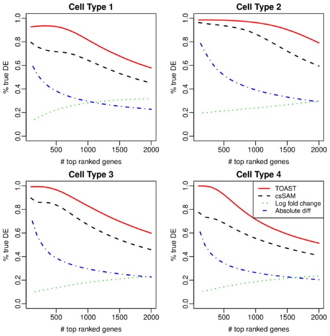
Comparison of csDE detection accuracy from simulation. Shown are the TDR curves, which plot the proportions of true discovery among top-ranked genes against the number of top-ranked genes. Methods under comparison include TOAST, csSAM, lfc and absolute difference

Due to the poor performances from log fold-change and absolute difference, we only focus on the comparison of csSAM and TOAST hereafter.

Impact of noise level and sample size

The noises in the data can come from two sources: (i) biological variation: the variation of pure cell-type profiles among different sample; and (ii) technical noise: the measurement error. Here, we investigate the impact of technical noise level and sample sizes on the performance of the proposed method.

Supplementary Figure S2 shows the TDR curves from the proposed method under different technical noise levels and sample sizes. We consider noise levels ranging from low (n_sd = 0.1, here n_sd is the parameter controls the magnitude of measurement error and is described in the Section 2) to high (n_sd = 10). Medium level (n_sd = 1) corresponds to the noise level estimated from the Immune Data (described in the Section 2), and is close to typical real data observations. We find that technical noise level has substantial influence on the performance of TOAST. When noise level is low, 50 samples in each group are enough for good performance. When noise level is very high, the method suffers significantly especially when sample size is small. In this case, larger sample size (500 samples in each group) can substantially improve the performance.

Impact of biological variation

We further evaluate the impact of biological variation (the within-group variation of pure cell-type profiles across subjects). Supplementary Figure S4 shows the TDR curves from TOAST under different levels of biological variation (controlled by n_ref, described in the Section 2). n_ref = 1 corresponds to the biological variance level estimated from the Immune Data. Similar to the technical noise, we find that the biological variation also has substantial impact on the performance of TOAST. This is expected, since greater biological variation reflects higher heterogeneity in samples, making it more challenging to detect csDE/csDM. Different from n_sd, which multiplies by the variance of a normal distribution, n_ref multiples by the standard deviation of a log-normal distribution. This leads to the results in Supplementary Figure S4 that, a small change in n_ref can substantially impact the variation of simulated reference panel. When biological variation is small (n_ref = 0.1), the TDR among the 2000 top-ranked genes is higher than 0.9 for all tissues. When biological variation is large (n_ref = 2), <50% of the 2000 top-ranked genes are true.

Impact of proportion magnitude

Results in Supplementary Figure S2 show that the orders of TDR curves from different hypothetical cell types are similar under all simulation settings, with the red curves being the highest in most cases. Further investigation reveals that this order is related to the abundance of each cell type in the mixture. As described in the Section 2, the simulated proportions are based on the proportion estimation of a real dataset (shown in Supplementary Fig. S3). In general, cell type 2 is the most abundant cell type, while cell type 4 is the rarest. So in simulation, cell type 2 has the best receiver operating characteristic curve on most occasions, and cell type 4 has the worst.

To further evaluate the impact of proportion in csDE detection, we conduct another simulation study with all procedures the same as described in the Section 2 except the proportion generation step. Instead of using real data estimated proportions, we generate proportions from $\mathit{Dirichlet}(590,300,100,10)$ for both cases and controls. This ensures the proportions of the first cell type are around 59% for all subjects, second around 30%, etc. Then the obtained TDRs can be linked to the average proportions of the corresponding cell types. In addition, we run simulations using true proportions as input for TOAST, i.e. no proportion estimation procedure involved, thus the impact of proportion estimation accuracy will be excluded. Figure 3a summarizes the distributions of true DE percentages in the top 2000 genes for four cell types, which have different proportions in the mixture. It shows that the magnitude of proportion is closely related with the detection performance. DE genes in cell types with smaller mixture proportions are much harder to be detected. This is expected, because the changes in cell types that make up a smaller proportion of the tissue have smaller contribution to the overall measurement, and thus are more difficult to be identified. To better detect csDE for rarer cell types, the only effective way is to increase the sample size.

Fig. 3.

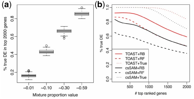
Impact of different factors on simulation results. (a) Impact of mixture proportion magnitude on detection accuracy. Boxplot of the detection accuracy (represented by the proportions of true DEs in the 2000 top-ranked genes) by different magnitude of mixture proportion values. $\sim 0.01$ means proportion magnitude around 1%. (b) Impact of proportion estimation on TOAST and csSAM in Cell Type 1. TDR curves comparing TOAST versus csSAM when different deconvolution methods are used as up-stream proportion estimation methods. RB: reference-based. RF: reference-free. True: true proportion

Impact of proportion estimation

Among all the factors, we find the accuracy of proportion estimation has vital impacts on the accuracy of csDE detection. We compared the performances of TOAST and csSAM, using different estimated proportions as inputs. The estimated proportions are from RB and RF methods. We also include the results using true proportions as benchmark.

The TDRs for csDE detection are shown in Figure 3b. In all scenarios, TOAST outperforms csSAM. Obviously, using the true proportion gives the best results for TOAST and csSAM. When using the estimated proportions, RB estimation provides better results than RF estimation. This is as expected, since RB method uses extra information (pure cell-type profiles), and was reported to produce better proportion estimation (Newman et al., 2015).

Impact of changes in multiple cell types

In the previous simulations, DE genes are randomly generated in each cell type. Even though by chance some genes have DE in two or more cell types simultaneously, it is still interesting to explicitly evaluate the performance of TOAST when DE occurs in multiple cell types. One real life example is aging, which is likely to alter genomic profiles in several cell types in the blood. Supplementary Figure S6 shows the TDR plots for detecting DE when two, three or four cell types simultaneously. This demonstrates that TOAST consistently provides the most accurate results.

Testing for other hypotheses

All the simulation results presented above are for testing difference of one cell type between cases and controls, i.e. the hypothesis 1 in Section 2.2. We also conduct additional simulations to examine the performance of TOAST on testing other hypotheses. In these simulations, we apply the Bioconductor package limma on the underlying reference panels, and define the genes with FDR < 0.05 as true DE genes. The detailed procedure of this experiment is described in Supplementary Materials (Section S2). Supplementary Figure S7 demonstrates the TDR of TOAST in detecting difference between two cell types in the normal group (hypothesis 2 in Section 2.2, Supplementary Fig. S7a), in the disease group (hypothesis 3 in Section 2.2, Supplementary Fig. S7b) and detecting difference of the changes between two cell types in two conditions (hypothesis 3 in Section 2.2, Supplementary Fig. S7c). We find that TOAST achieves good performance in all these settings.

Computational performance

TOAST provides superior computational performance since it is based on linear regression. csSAM, on the other hand, relies on permutation procedure and is much more computationally demanding. We benchmark the computational performances of TOAST and csSAM on a laptop computer with 4GB RAM and Intel Core i5 CPU. For a moderate dataset with 20 000 genes and 100 samples in each group, one csDE call from TOAST takes 1.42 s, but 378.67 s from csSAM. Thus, TOAST is 266 times faster than csSAM.

Overall, the simulation studies demonstrate that our proposed method TOAST provides more accurate and efficient performance in detecting cell-type specific changes compared to csSAM. We find that the most important factor in the csDE/csDM detection accuracy is the proportion estimation, which is strongly influenced by the technical noise. Moreover, cell types with lower proportions are more difficult to analyze, since their signal in the mixed data is lower.

3.2 Real data results

Application to immune dataset

We use this dataset to showcase the capability of TOAST in detecting differences among cell types within the same group (hypothesis 2 of Section 2.2). The specific goal of this data analysis is to detect DE genes for pair-wise comparisons of two different cell lines using the mixture data only, e.g. the DE genes between Jurkat and IM-9, IM-9 and THP-1, etc. It is worth noting that we do not compare csSAM in this application because csSAM does not provide the function of detecting DE genes across cell types under the same condition. For each comparison, we define the gold standard based on the pure cell line profiles. We apply limma (Ritchie et al., 2015) on the pure cell line profiles to call DE genes. The true DE genes are defined as the ones with (i) the limma P-value smaller than 0.05; and (ii) the absolute lfc ≥3. The non-DE genes are defined as the ones with limma P-value >0.8. We do not include the genes that have P-values between 0.05 and 0.8 to avoid ambiguity.

Using mixture proportions estimated from RB method, we apply TOAST on the mixed data to detect DE genes for all pair-wise comparisons. Figure 4a shows the TDR curves for all comparisons. Overall, the proposed method demonstrates good accuracy. The TDR for three of the comparisons are over 80% for the top 500 genes. The results for comparing IM-9 and THP-1 are the worst. To further investigate these results, we show the correlation of estimated versus true proportions in Figure 4b. The proportion estimation is the worst for IM-9 and THP-1. This partly explains the bad results from IM-9 versus THP-1 comparison. We further try to use RF method to estimate the mixing proportions, and use these estimates as input for DE detection. The results are shown in Supplementary Figure S9a. Overall, these results are much worse than using the RB proportion estimates. We also use the true proportion as inputs (Supplementary Fig. S10), which yields good accuracy for all comparisons. These results suggest that our proposed method can satisfactorily detect DE genes across cell types from mixed sample data, and that the detection accuracy is highly dependent on the accuracy of proportion estimation. These conclusions are consistent with the simulation results.

Fig. 4.

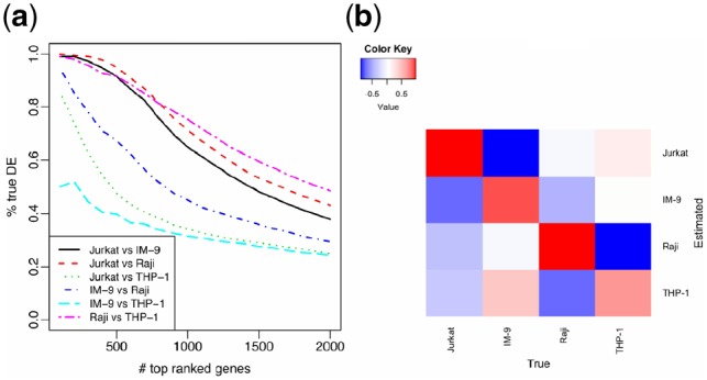
Accuracy of detecting DE across cell types in the Immune Dataset using TOAST. (a) TDR curves for pair-wise comparisons of different cell types using TOAST. RB with 1000 reference genes is used to estimate proportions. (b) Heatmap of Pearson’s correlation coefficients between the estimated versus true mixture proportions

Application to human brain methylation data

We use the dataset GSE41826 to show the functionality of TOAST in detecting cell-type specific changes among different groups (hypothesis 1 of Section 2.2). The dataset contains pure and mixed samples for a number of individuals with different genders. The original study aimed to identify differences between patients with major depression and healthy controls but did not find significant cell-type specific changes after adjusting for multiple comparison (Guintivano et al., 2013). Our analysis confirms their findings in that contrast. We do find a reasonable set of DMCs between males and females with low false discovery rate, which we use to benchmark the methods for detecting cell-specific differences.

We first group the healthy samples from GSE41826 by gender. We construct gold standard DMC using profiles of sorted neuron and glia. We apply Bioconductor package minfi (Aryee et al., 2014) to call DMCs between the pure cell-type profiles of neuron and glia. True DMC is defined as false discovery rate smaller than 0.05, which results in 9439 and 9337 true DMCs (out of 480 491 CpGs) in neuron and glia, respectively. Here true DMC in neurons include all DMC detected in pure neurons, not just the ones exclusively identified in neurons, likewise for true DMC in glia. Non-DM sites are defined as those with false discovery rate larger than 0.8. The DM and non-DM sites are then used as benchmark to evaluate the csDM calling from whole-tissue sample data. We estimate the proportions (for neuron and glia) from the whole-tissue DNA methylation data with RB deconvolution. The whole-tissue DNA methylation data of five healthy males and five healthy females and the estimated mixture proportions are used as inputs to both TOAST and csSAM. The TDR curves for the results are shown in Figure 5. Overall, these results are not very accurate, because of small sample size and high inter-individual heterogeneity even for the pure tissue profile. However with the same input data, the proposed method still provides much higher accuracy among the top CpG sites than csSAM.

Fig. 5.

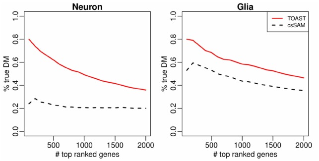
Accuracy of detecting csDM in Human brain methylation data. TDR curves for csDM detection from the comparisons of healthy males versus healthy females in Neuron and Glia, using TOAST and csSAM. RB with 1000 reference genes is used to estimate mixture proportions

It is important to note that csSAM is not designed for DNA methylation data analysis. However, the two-step algorithm (solve for pure tissue profiles and then perform test) can be applied to methylation data as well. The result here shows that the proposed framework performs better than the two-step approach.

The example above, based on human brain DNA methylation data, involves only two cell types. We chose this data example due to the difficulty of obtaining public dataset involving more cell types with ground truth for assessment. Nonetheless, to illustrate the application in tissues with more cell types, we include an example in the Supplementary Material (Section S5 and Supplementary Fig. S12), using a DNA methylation dataset from HIV patients and controls from GEO with accession number GSE67705 (Gross et al., 2016).

4 Discussion

In this work, we develop a general statistical framework named ‘TOAST’ to account for sample mixing and detect cell–type specific differential features. By ‘cell-type specific’ differential effects we, like others (Kuhn et al., 2011; Montaño et al., 2013; Shen-Orr et al., 2010; Westra et al., 2015; Zheng et al., 2018), refer to within-cell-type differences as opposed to marginal differences. The method is based on simple but rigorous statistical modeling, and provides flexible functionalities for testing a variety of cell-type specific differences. A number of previous methods also utilize linear model and are similar in spirit to our method. As shown in the Supplementary Materials (Section S6), these methods are simplified version or special cases of our framework. Compared with csSAM, which performs statistical test on deconvolved pure cell-type signals, TOAST can be considered as jointly performing signal deconvolution and hypothesis testing. These results in improved performance, evidenced by simulation and real data analyses. The proposed method can potentially be applied to a number of high-throughput experiments, including but not limited to gene expression microarray data, DNA methylation 450K data, proteomics data, etc.

The simulation and real data analyses presented in this work are mostly focused on (gene expression or methylation) microarray data, where the data can be approximated by log-normal distribution. We also conduct additional simulations for RNA-seq data, and demonstrate that the proposed method performs well in detecting csDE in RNA-seq (details are provided in Supplementary Material Section S3 and Supplementary Fig. S8). However, one caveat of such analysis is that the deconvolution method for RNA-seq data is still not well developed and tested. It is not yet clear how one can obtain accurate estimates of the mixing proportions, which is an important prerequisite for the good performance of cell-type specific analysis and something we plan to do in the near future.

In the simulations, we generate individualized reference panels by adding noise randomly. When the reference panel and population under study have systematic discrepancy (in age, ethnic group, etc.), there could be bias. However, this would only affect proportion estimation, not differential signal detection. Since estimating cell-type proportion is not the main goal of this work and the proportions are assumed to be given, such discrepancy would not have impact on the proposed method. This being said, we believe that a careful examination of deconvolution methods with the consideration of systematical discrepancy between the reference panel and observations is an important problem to investigate.

There has been some discussion about whether one should use raw- or log-scale data in signal deconvolution and differential analysis, including opinions arguing for using raw scale data (Abbas et al., 2009; Gong et al., 2011; Zhong et al., 2013; Zhong and Liu, 2012) and for using log transformed data (Gaujoux and Seoighe 2013). Theoretically, mixing takes place at the raw scale and linear deconvolution is expected to work on the same scale. However, real biological data from high-throughput technology are complex and often include many sources of noise, distortion and anomaly that cannot be fully captured by simple parametric simulation. The benefit of resistance to outliers often is a worthwhile tradeoff for the loss of perfect linear relationship in between the mixed and latent cell-type specific measures of expression/methylation. As a result, real data applications may find that analyzing the log-scale data delivers similar or even better performance (Supplementary Fig. S11). We include a more in-depth discussion on this topic in Supplementary Section S4. The implementation of the TOAST software allows the user to opt for either raw- or log-scale data.

Whilst our paper was under review, we became aware of the publication of a similar method called CellDMC (Zheng et al., 2018). The data modeling framework of CellDMC is largely equivalent to TOAST, but it works for the first hypothesis test (cell-type specific changes associated with the outcome). TOAST enables more flexible hypothesis testing depending on the scientists’ interest. Though we expect that the most common goal is identifying differential effects within the cell type(s) of interest (as CellDMC does), one may also be interested in whether differences are unique to a cell type (i.e. qualitatively different across cell types, with ${\beta }_k\ne 0$ for only one cell type), or to different extent across cell types (i.e. quantitatively different across cell types, with ${\beta }_p-{\beta }_q\ne 0$). The combined linear model in TOAST allows the user to define the hypothesis of interest, and the flexibility is one of the advantages of using TOAST. In addition, CellDMC was tested exclusively on DNA methylation data, while we show that TOAST is also applicable on mRNA expression datasets.

We anticipate several natural extensions of TOAST. First, the essence of the data modeling and statistical inference from our proposed method can be applied to other types of high-throughput data such as ChIP-seq or bisulfite-sequencing, even though the detailed model fitting and statistical testing strategies will be different. Secondly, we currently model the effect of covariate in a linear system. It is possible that some covariates (such as age) have a non-linear effect. In this case, we can replace covariates Z by $f(\mathit{Z})$ to model the non-linear effect, where f can be a parametric or non-parametric function.

References

- Abbas A.R. et al. (2009) Deconvolution of blood microarray data identifies cellular activation patterns in systemic lupus erythematosus. PLoS One, 4, e6098.. [DOI] [PMC free article] [PubMed] [Google Scholar]
- Anders S., Huber W. (2010) Differential expression analysis for sequence count data. Genome Biol., 11, R106.. [DOI] [PMC free article] [PubMed] [Google Scholar]
- Aryee M.J. et al. (2014) Minfi: a flexible and comprehensive Bioconductor package for the analysis of infinium DNA methylation microarrays. Bioinformatics, 30, 1363–1369. [DOI] [PMC free article] [PubMed] [Google Scholar]
- Basu S. et al. (2010) Purification of specific cell population by fluorescence activated cell sorting (FACS). J. Vis. Exp., 41, 1546. [DOI] [PMC free article] [PubMed] [Google Scholar]
- Bennett D.A. et al. (2005) The rush memory and aging project: study design and baseline characteristics of the study cohort. Neuroepidemiology, 25, 163–175. [DOI] [PubMed] [Google Scholar]
- Brunet J.-P. et al. (2004) Metagenes and molecular pattern discovery using matrix factorization. Proc. Natl. Acad. Sci. USA, 101, 4164–4169. [DOI] [PMC free article] [PubMed] [Google Scholar]
- Clarke J. et al. (2010) Statistical expression deconvolution from mixed tissue samples. Bioinformatics, 26, 1043–1049. [DOI] [PMC free article] [PubMed] [Google Scholar]
- ENCODE Project Consortium (2012) An integrated encyclopedia of DNA elements in the human genome. Nature, 489, 57.. [DOI] [PMC free article] [PubMed] [Google Scholar]
- Erkkilä T. et al. (2010) Probabilistic analysis of gene expression measurements from heterogeneous tissues. Bioinformatics, 26, 2571–2577. [DOI] [PMC free article] [PubMed] [Google Scholar]
- Feng H. et al. (2014) A Bayesian hierarchical model to detect differentially methylated loci from single nucleotide resolution sequencing data. Nucleic Acids Res., 42, e69–e69. [DOI] [PMC free article] [PubMed] [Google Scholar]
- Gaujoux R., Seoighe C. (2013) CellMix: a comprehensive toolbox for gene expression deconvolution. Bioinformatics, 29, 2211–2212. [DOI] [PubMed] [Google Scholar]
- Gaujoux R., Seoighe C. (2010) A flexible r package for nonnegative matrix factorization. BMC Bioinformatics, 11, 367.. [DOI] [PMC free article] [PubMed] [Google Scholar]
- Gong T. et al. (2011) Optimal deconvolution of transcriptional profiling data using quadratic programming with application to complex clinical blood samples. PLoS One, 6, e27156.. [DOI] [PMC free article] [PubMed] [Google Scholar]
- Gross A.M. et al. (2016) Methylome-wide analysis of chronic HIV infection reveals five-year increase in biological age and epigenetic targeting of HLA. Mol. Cell, 62, 157–168. [DOI] [PMC free article] [PubMed] [Google Scholar]
- Guintivano J. et al. (2013) A cell epigenotype specific model for the correction of brain cellular heterogeneity bias and its application to age, brain region and major depression. Epigenetics, 8, 290–302. [DOI] [PMC free article] [PubMed] [Google Scholar]
- Houseman E.A. et al. (2012) DNA methylation arrays as surrogate measures of cell mixture distribution. BMC Bioinformatics, 13, 86.. [DOI] [PMC free article] [PubMed] [Google Scholar]
- Houseman E.A. et al. (2014) Reference-free cell mixture adjustments in analysis of DNA methylation data. Bioinformatics, 30, 1431–1439. [DOI] [PMC free article] [PubMed] [Google Scholar]
- Houseman E.A. et al. (2016) Reference-free deconvolution of DNA methylation data and mediation by cell composition effects. BMC Bioinformatics, 17, 259.. [DOI] [PMC free article] [PubMed] [Google Scholar]
- Itagaki S. et al. (1989) Relationship of microglia and astrocytes to amyloid deposits of Alzheimer disease. J. Neuroimmunol., 24, 173–182. [DOI] [PubMed] [Google Scholar]
- Jaffe A.E., Irizarry R.A. (2014) Accounting for cellular heterogeneity is critical in epigenome-wide association studies. Genome Biol., 15, R31.. [DOI] [PMC free article] [PubMed] [Google Scholar]
- Kalaria R.N. (1999) Microglia and Alzheimer’s disease. Curr. Opin. Hematol., 6, 15.. [DOI] [PubMed] [Google Scholar]
- Kuhn A. et al. (2011) Population-specific expression analysis (PSEA) reveals molecular changes in diseased brain. Nat. Methods, 8, 945.. [DOI] [PubMed] [Google Scholar]
- Liu Y. et al. (2013) Epigenome-wide association data implicate DNA methylation as an intermediary of genetic risk in rheumatoid arthritis. Nat. Biotechnol., 31, 142–147. [DOI] [PMC free article] [PubMed] [Google Scholar]
- Maragakis N.J., Rothstein J.D. (2006) Mechanisms of disease: astrocytes in neurodegenerative disease. Nat. Rev. Neurol., 2, 679.. [DOI] [PubMed] [Google Scholar]
- Montaño C.M. et al. (2013) Measuring cell-type specific differential methylation in human brain tissue. Genome Biol., 14, R94.. [DOI] [PMC free article] [PubMed] [Google Scholar]
- Newman A.M. et al. (2015) Robust enumeration of cell subsets from tissue expression profiles. Nat. Methods, 12, 453.. [DOI] [PMC free article] [PubMed] [Google Scholar]
- Repsilber D. et al. (2010) Biomarker discovery in heterogeneous tissue samples-taking the in-silico deconfounding approach. BMC Bioinformatics, 11, 27.. [DOI] [PMC free article] [PubMed] [Google Scholar]
- Ritchie M.E. et al. (2015) limma powers differential expression analyses for RNA-sequencing and microarray studies. Nucleic Acids Res., 43, e47. [DOI] [PMC free article] [PubMed] [Google Scholar]
- Schmitz B. et al. (1994) Magnetic activated cell sorting (MACS) a new immunomagnetic method for megakaryocytic cell isolation: comparison of different separation techniques. Eur. J. Haematol., 52, 267–275. [DOI] [PubMed] [Google Scholar]
- Shen-Orr S.S. et al. (2010) Cell type–specific gene expression differences in complex tissues. Nat. Methods, 7, 287.. [DOI] [PMC free article] [PubMed] [Google Scholar]
- Sonnen J.A. et al. (2009) Neuropathology in the adult changes in thought study: a review. J. Alzheimers Dis., 18, 703–711. [DOI] [PMC free article] [PubMed] [Google Scholar]
- Teschendorff A.E. et al. (2017) A comparison of reference-based algorithms for correcting cell-type heterogeneity in epigenome-wide association studies. BMC Bioinformatics, 18, 105.. [DOI] [PMC free article] [PubMed] [Google Scholar]
- Tusher V.G. et al. (2001) Significance analysis of microarrays applied to the ionizing radiation response. Proc. Natl. Acad. Sci. USA, 98, 5116–5121. [DOI] [PMC free article] [PubMed] [Google Scholar]
- Urenjak J. et al. (1993) Proton nuclear magnetic resonance spectroscopy unambiguously identifies different neural cell types. J. Neurosci., 13, 981–989. [DOI] [PMC free article] [PubMed] [Google Scholar]
- Verkhratsky A. et al. (2010) Astrocytes in Alzheimer’s disease. Neurotherapeutics, 7, 399–412. [DOI] [PMC free article] [PubMed] [Google Scholar]
- Westra H.-J. et al. (2015) Cell specific eQTL analysis without sorting cells. PLoS Genet., 11, e1005223.. [DOI] [PMC free article] [PubMed] [Google Scholar]
- Wu H. et al. (2012) A new shrinkage estimator for dispersion improves differential expression detection in RNA-seq data. Biostatistics, 14, 232–243. [DOI] [PMC free article] [PubMed] [Google Scholar]
- Zheng S.C. et al. (2018) Identification of differentially methylated cell types in epigenome-wide association studies. Nat. Methods, 15, 1059.. [DOI] [PMC free article] [PubMed] [Google Scholar]
- Zhong Y., Liu Z. (2012) Gene expression deconvolution in linear space. Nat. Methods, 9, 8.. [DOI] [PubMed] [Google Scholar]
- Zhong Y. et al. (2013) Digital sorting of complex tissues for cell type-specific gene expression profiles. BMC Bioinformatics, 14, 89. [DOI] [PMC free article] [PubMed] [Google Scholar]
- Zou J. et al. (2014) Epigenome-wide association studies without the need for cell-type composition. Nat. Methods, 11, 309–311. [DOI] [PubMed] [Google Scholar]
Associated Data
This section collects any data citations, data availability statements, or supplementary materials included in this article.