Maximum Entropy Framework for Predictive Inference of Cell Population Heterogeneity and Responses in Signaling Networks

Abstract

Predictive models of signaling networks are essential for understanding cell population heterogeneity and designing rational interventions in disease. However, using computational models to predict heterogeneity of signaling dynamics is often challenging because of the extensive variability of biochemical parameters across cell populations. Here, we describe a maximum entropy-based framework for inference of heterogeneity in dynamics of signaling networks (MERIDIAN). MERIDIAN estimates the joint probability distribution over signaling network parameters that is consistent with experimentally measured cell-to-cell variability of biochemical species. We apply the developed approach to investigate the response heterogeneity in the EGFR/Akt signaling network. Our analysis demonstrates that a significant fraction of cells exhibits high phosphorylated Akt (pAkt) levels hours after EGF stimulation. Our findings also suggest that cells with high EGFR levels predominantly contribute to the subpopulation of cells with high pAkt activity. We also discuss how MERIDIAN can be extended to accommodate various experimental measurements.

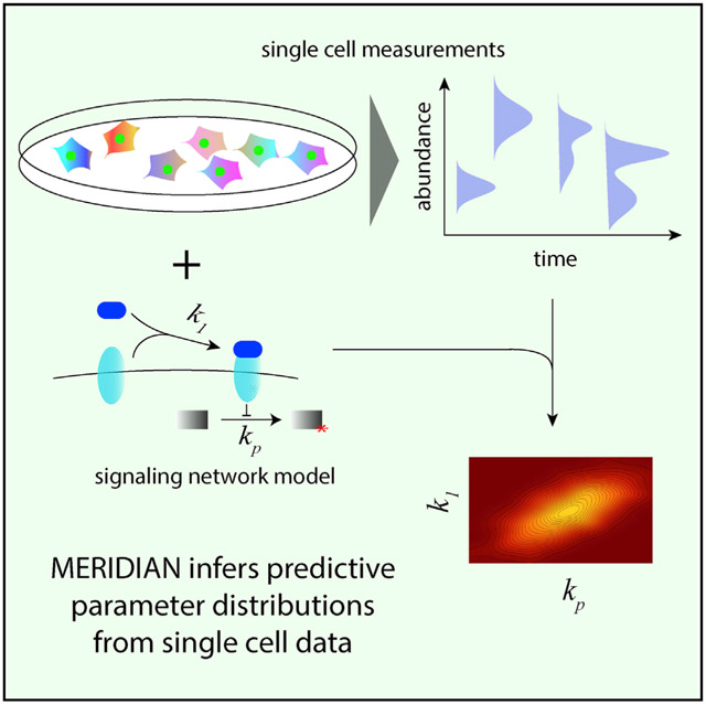
Graphical Abstract

In Brief

Dixit et al. describe MERIDIAN, a nonparametric maximum entropy-based framework to infer predictive signaling-network parameter distributions from single-cell data. Using this framework, they analyze population heterogeneity in phosphorylation cascades downstream of growth factors.

INTRODUCTION

Signaling cascades in genetically identical cells often respond to extracellular stimuli in a heterogeneous manner (Raj and van Oudenaarden, 2008). This heterogeneity arises largely because of cell-to-cell variability in biochemical signaling parameters, such as reaction rates and chemical species abundances (Albeck et al., 2008; Spencer et al., 2009; Meyer et al., 2012; Llamosi et al., 2016; Kallenberger et al., 2017). The response variability across cells can have important functional consequences, for example, in multimodal developmental decisions (Chastanet et al., 2010) and fractional killing of cancer cells treated with chemotherapeutic compounds (Albeck et al., 2008; Spencer et al., 2009, Gerosa et al., 2019). Therefore, the ability to predict heterogeneity in cell populations is important for predicting heterogeneous outcomes of biological stimulations and in designing rational intervention in disease states (Niepel et al., 2009).

Several experimental techniques such as flow cytometry, immunofluorescence (Wu and Singh, 2012), and live cell assays (Meyer et al., 2012) have been developed to investigate the cell-to-cell variability of biochemical species abundances. However, it is often difficult to estimate the distribution of biochemical parameters consistent with these experimental measurements. The reasons for this challenge are primarily 3-fold. First, biochemical parameters such as protein abundances and reaction rates vary substantially across cells in a population (Raj and van Oudenaarden, 2008). For example, previous studies have reported the coefficients of variation of protein abundances in the range of 0.1–0.6 (Niepel et al., 2009). Consequently, effective rates of signaling reactions also vary substantially between cells (Chung et al., 1997; Meyer et al., 2012). Second, multivariate parameter distributions can potentially have complex shapes. For example, abundance distributions of key signaling proteins and enzyme often exhibit multimodality (Frei et al., 2016). Finally, available single-cell measurements are typically not sufficient to uniquely infer the underlying parameter variability—the challenge usually referred to as “parameter non-identifiability” (Banks et al., 2012).

Over the last decade, several computational methods have been developed to estimate the joint distribution of parameters consistent with experimentally measured cell-to-cell variability of biochemical species (Waldherr et al., 2009; Hasenauer et al., 2011, 2014; Zechner et al., 2012, 2014; Loos et al., 2018; Waldherr, 2018; Loos and Hasenauer, 2019). Most of these methods circumvent the ill-posed inverse problem of estimation of the parameter distribution (Banks et al., 2012) by making specific ad hoc choices about the underlying distribution. For example, Hasenauer et al. (2011, 2014) (see also (Waldherr et al., 2009; Loos et al., 2018) approximate the parameter distribution as a linear combination of predefined functions. Waldherr et al. 2009 approximate the parameter distribution using Latin hypercube sampling (LHS). Similarly, (Zechner et al. (2012, 2014) assume that the parameters are distributed according to a log-normal or gamma distribution. The limitations arising due to these specific choices of parameter distributions remain unknown.

Building on our previous work (Dixit, 2013; Eydgahi et al., 2013), we developed MERIDIAN, a maximum entropy-based framework for inference of heterogeneity in dynamics of signaling networks. Instead of enforcing a specific functional form of the parameter distribution a priori, MERIDIAN uses data-derived constraints to derive it de novo. The maximum entropy principle (Dixit et al., 2018) was first introduced more than a century ago in statistical physics. Notably, later work established the maximum entropy approach as an inference method with principled axiomatic justifications (Shore and Johnson, 1980). Among all candidate distributions that agree with the imposed constraints, the maximum entropy approach selects the one with the least amount of biases. Maximum entropy-based approaches have been successfully applied to a variety of biological problems, including protein structure prediction (Weigt et al., 2009), protein sequence evolution (Mora et al., 2010), neuron firing dynamics (Schneidman et al., 2006), molecular simulations (Dixit et al., 2015; Tiwary and Berne, 2016), and dynamics of biochemical reaction networks (Dixit, 2018).

In the paper, following a description of the key ideas behind MERIDIAN, we illustrate its performance using synthetic data. We then use MERIDIAN to study the heterogeneity in the signaling network leading to phosphorylation of protein kinase B (Akt). Epidermal growth factor (EGF)-induced Akt phosphorylation governs key intracellular processes (Manning and Toker, 2017) including metabolism, apoptosis, and cell cycle entry. Because of its central role in mammalian signaling, aberrations in the Akt pathway are implicated in multiple disorders (Manning and Toker, 2017). We apply MERIDIAN to infer the distribution over signaling parameters using previously collected experimental data on phosphorylated Akt (pAkt) (Lyashenko et al., 2018) and data on cell surface EGF receptor (sEGFR) abundance measured in MCF10A cells. We demonstrate that the parameter distribution inferred using MERIDIAN allows us to accurately predict the cell-to-cell heterogeneity of pAkt levels at late time points after stimulation as well as the heterogeneity of sEGFRs in response to EGF signal. Finally, we discuss possible generalizations of the developed framework to accommodate various experimental measurements.

RESULTS

Outline of MERIDIAN

We consider a signaling network comprising N chemical species whose intracellular abundances we denote by $\overline{x}=\{x_1,x_2,\dots ,x_N\}$. We assume that the molecular interactions among the species are described by a system of ordinary differential equations

$$\frac{d}{dt}\overline{x}(t,\overline{\theta })=f(\overline{x},\overline{\theta })$$ (Equation 1)

where $f(\overline{x},\overline{\theta })$ is a function of species abundances $\overline{x}$ and $\overline{\theta }=\{{\theta }_1,{\theta }_2,\dots \}$ is a vector of parameters describing the dynamics of the signaling networks. We denote by $x_a(t,\overline{\theta })$ the solution of Equation 1 for species “a” at time t with specific parameters $\overline{\theta }$, which we assume to vary across cells.

The MERIDIAN inference approach is illustrated in Figure 1. We use experimentally measured cell-to-cell variability of protein species “a” at multiple experimental conditions, for example, several time points (illustrated by histograms in Figure 1), to constrain the parameter distribution $P(\overline{\theta })$. Specifically, we first quantify the experimentally measured biochemical species variability by estimating bin fractionsφ_ik. In our notation, the index i specifies the experimental measurement, for example, measurement time and measured species, and k indicates the abundance distribution bin number for a given condition. Every distinct dynamical trajectory $x_a(t,\overline{\theta })$ (illustrated by red and blue curves in Figure 1) generated by specific parameter values $\overline{\theta }$ passes through a unique set of abundance bins (red curve through red bins and blue curve through blue bins in Figure 1) at multiple experimental conditions. Using MERIDIAN, we find a corresponding probability distribution $P(\overline{\theta })$ over parameters such that the corresponding distribution over dynamic trajectories $P[x_a(t,\overline{\theta })]$ is consistent with all experimentally measured abundance bin fractions. Below, we present the approach that we use to derive the functional form of $P(\overline{\theta })$.

Figure 1. Illustration of the MERIDIAN Inference Approach.

Cell-to-cell abundance variability of protein “a” is measured at four time points t₁, t₂, t₃, and t₄. From the single cell data, we determine the fraction ϕ_ik of cells that populate the k^th abundance bin in the i^th experimental measurement (time). The histograms show ϕ_ik across multiple experimental measurements. We find $P(\overline{\theta })$ using the maximum entropy approach while requiring that the corresponding distribution $P[{\mathit{x}}_a(t,\overline{\theta })]$ over dynamic trajectories of ${\mathit{x}}_a(t,\overline{\theta })$ simultaneously reproduces all experimentally measured abundance bin fractions.

Derivation of $P(\overline{\theta })$ using MERIDIAN

For simplicity, we first consider the case when the distribution of cell-to-cell variability in one species x_a is available only at a single time point t (for example, t = t₁ in Figure 1). We denote by $\overline{\varphi }=\{{\varphi }_1,{\varphi }_2,\dots ,{\varphi }_B\}$ the fraction of cells whose experimental measurement of x_a lies in individual abundance bins (numbered from 1 to B). Here, given that we are considering only one experimental measurement, we use, for brevity, only one index to indicate the bin fractions. We also assume that there are no experimental errors in determining $\overline{\varphi }$. Later, we demonstrate how it is possible to incorporate known experimental errors both in the inference procedure and in making predictions using $P(\overline{\theta })$.

Given a parameter distribution $P(\overline{\theta })$, the predicted fractions $\overline{\psi }=\{{\psi }_1,{\psi }_2,\dots ,{\psi }_B\}$ can be obtained as follows. Using Markov chain Monte Carlo (MCMC), we generate multiple parameter sets $\overline{\theta }$ from $P(\overline{\theta })$. For each $\overline{\theta }$, we solve Equation 1 and find $x_a(t,\overline{\theta })$, i.e., the predicted value of the species abundance at time t. Then, using the samples from the ensemble of trajectories, we estimate the predicted ψ_k as the fraction of sampled trajectories for which $x_a(t,\overline{\theta })$ passed through the k^th bin. Mathematically:

$${\psi }_k=\int I_k\left(x_a(t,\overline{\theta })\right)P(\overline{\theta })d\overline{\theta }$$ (Equation 2)

where I_k(x) is an indicator function i.e., I_k(x) is equal to one if x lies in the k^th bin and zero otherwise.

The central idea behind MERIDIAN is to find the maximum entropy distribution $P(\overline{\theta })$ over parameters such that all predicted fractions ψ_k agree with those from experimental measurements, φ_k. Formally, we seek $P(\overline{\theta })$ with the maximum entropy

$$S=-\int P(\overline{\theta })\log \frac{P(\overline{\theta })}{q(\overline{\theta })}d\overline{\theta }$$ (Equation 3)

subject to normalization $(\int P(\overline{\theta })d\overline{\theta }=1)$ and data-derived constraints ψ_k = φ_k for all k. Here, $q(\overline{\theta })$ plays a role similar to the prior distribution in Bayesian statistics (Caticha and Preuss, 2004). In this work, we choose $q(\overline{\theta })$ to be a uniform distribution within literature-derived ranges of parameters, but other choices can be used as well.

To impose aforementioned constraints and perform the entropy maximization, we use the method of Lagrange multipliers. To that end, we write the Lagrangian function

$$L=S+\eta \left(\int P(\overline{\theta })d\overline{\theta }-1\right)-\sum _{k=1}^B{\lambda }_k\left(\int I_k\left(x_a(t,\overline{\theta })\right)P(\overline{\theta })d\overline{\theta }-{\varphi }_k\right)$$ (Equation 4)

where η is the Lagrange multiplier associated with normalization and λ_k are the Lagrange multipliers associated with bin fractions φ_k. By differentiating Equation 4 with respect to $P(\overline{\theta })$ and setting the derivative to zero, we obtain the Gibbs-Boltzmann form:

$$P(\overline{\theta }\mid \overline{\lambda })=\frac{1}{\Omega }q(\overline{\theta })\text{exp}\left(-\sum _{k=1}^B{\lambda }_k{I}_k\left(x_a(t,\overline{\theta })\right)\right),$$ (Equation 5)

where Ω is the partition function that normalizes the probability distribution. Equation 5 is a key conceptual foundation of this work. We use it to estimate the parameter distribution based on user-specified constraints.

The aforementioned derivations are restricted to using single-cell data measured at one time point. In the STAR Methods, we discuss the generalization of the approach when abundances of multiple species are measured at several time points. The details of the convex numerical optimization problem of Lagrange multipliers, MERIDIAN-based predictions, and possible generalizations of MERIDIAN to accommodate various experimental measurements can also be found in the STAR Methods.

Finally, we note that given the high-dimensional nature of the parameter space, in many computational models of biological systems, the collected data are usually not sufficient to fully constrain the multidimensional parameter distribution (Banks et al., 2012). As a result, the parameter distribution inferred by MERIDIAN reflects both the true biological variability in parameters as well as parameter non-identifiability. Moreover, the relative contribution of non-identifiability to the inferred parameter distribution will likely increase with an increase in the dimensionality of the parameter space.

MERIDIAN Performance on Synthetic Data

Before applying MERIDIAN to investigate experimentally measured cell-to-cell variability, we decided to first validate the approach with synthetic data. To that end, we used a previously published model of the EGFR/Akt pathway (Chen et al., 2009) to generate in silico single-cell data for five different perturbations of the pathway. These perturbations represented several known cancer-related pathologies of the signaling network. Using the pathway model, we then investigated whether MERIDIAN can accurately predict single-cell distributions of biochemical species by comparing the predicted distributions with synthetically generated single-cell data.

Computational Model of the EGFR/Akt Signaling Network

Signal transduction in the EGFR/Akt network is illustrated in Figure 2. Following stimulation of cells with EGF, it binds to cell surface EGFRs (sEGFRs). Ligand-bound receptors then dimerize with other ligand-bound receptors as well as ligand-free receptors. EGFR dimers phosphorylate each other, and phosphorylated receptors (active receptors, pEGFRs) on the cell surface lead to downstream phosphorylation of Akt (pAkt). Both active and unphosphorylated (inactive) receptors are internalized with different rates from the cell surface because of receptor endocytosis. After addition of EGF to the extracellular medium, pAkt levels first increase transiently within minutes and then, as a result of receptor endocytosis, both pAkt and sEGFR levels decrease within hours after EGF stimulation (Chen et al., 2009).

Figure 2. Illustration of the EGF/EGFR Pathway Leading to Phosphorylation of Akt.

Extracellular EGF (red disc) binds to cell surface EGFRs leading to their dimerization. Dimerized EGFRs are autophosphorylated and lead to phosphorylation of Akt. Active and inactive receptors are removed from the cell surface through internalization into endosomes. Asterisk represents phosphorylation and the rate constants marked with an asterisk are associated with phosphorylated receptors. We only show a subset of all interactions in the model. See STAR Methods for details of the corresponding computational model.

To explore the cell-to-cell variability in this pathway, we used a dynamical model of EGF/EGFR dependent Akt phosphorylation based on (Chen et al. 2009). The model (see Figure 2) includes reactions describing EGF binding to EGFR and subsequent receptor dimerization, phosphorylation, dephosphorylation, internalization, and degradation. To keep the model relatively small, we simplified pEGFR-dependent pAkt activation by assuming a single-step activation of Akt by pEGFR (STAR Methods). The first and second order rate constants used in the model should be treated as effective rates, given that the law of mass action is only an approximation to the complex interactions in the EGFR/Akt pathway. The pathway model we used had 17 chemical species and 20 parameters. See Table S1 for the list of model parameters and Table S2 for the list of model variables. The model equations are given in the STAR Methods.

Parameter Inference Using Synthetic Data

Using synthetic multivariate parameter distributions, we generated in silico data for five different EGFR pathway parameterizations. The first parameterization represented the wild-type state of the network in MCF10A cells. Next, we simulated four different perturbations to the synthetic parameter distribution to represent four common cancer-related pathway pathologies. Specifically, we simulated (1) EGFR overexpression (Herbst, 2004), by increasing the rate of EGFR delivery to the cell surface, (2) PTEN loss (Martini et al., 2014), by decreasing the rate of dephosphorylation of pAkt, (3) decrease in EGFR downregulation, by decreasing the rate of endocytosis of activated EGFRs (Tomas et al., 2014), and (4) decrease in EGFR phosphatase activity, by reducing the rate of EGFR dephosphorylation (Tiganis, 2002) (see STAR Methods).

For each of these five parameterizations, we generated single-cell data (for ~4 × 10⁴ in silico single cells) describing (1) pAkt levels at 0, 5, 15, 30, and 45 min after stimulation with 0.1, 0.31, 3.16, 10, and 100 ng/ml of EGF and (2) steady-state sEGFR levels after prolonged stimulation with 0, 1, and 100 ng/ml of EGF (180 min) (STAR Methods). These 24 synthetic single-cell distributions (21 pAkt distributions and 3 sEGFR distributions) were each binned into 15 bins. The bin sizes and locations were chosen to cover the entire range of the observed variability (Table S3) and a total of 15 × 24 = 360 bin fractions $\overline{\varphi }$ were obtained. Next, for each aforementioned parameterization, we inferred the joint parameter distribution of the EGFR pathway by optimizing the 360 Lagrange multipliers using MERIDIAN (STAR Methods; Figures S1-S5).

Prediction of Single-Cell Dynamics Using the Inferred Distribution

Using the inferred parameter distribution, we next investigated whether single cell pAkt distributions at early times after stimulation (up to 45 min of continuous EGF stimulation) could predict the late time steady-state distributions of pAkt levels. To that end, using the synthetic parameter distributions for each of the five parameterizations, we sampled ~4 × 10⁴ parameter sets and simulated single-cell pAkt levels after 3 h of EGF stimulation across multiple EGF doses. These represented the synthetic in silico data against which we tested the MERIDIAN-based predictions. The MERIDIAN predictions were generated by sampling ~4 × 10⁴ parameter sets from the inferred parameter distributions (STAR Methods).

Notably, the mean values and standard deviations of pAkt levels were accurately predicted by MERIDIAN across all five realizations (the means and the standard deviations of steady-state pAkt levels were within ~7% of the in silico data, comparable to the prediction accuracy with real data, see below). As shown in Figures 3A-3C and S6, MERIDIAN accurately predicted single-cell pAkt distributions for all five parameterizations of the pathway and across two orders of magnitude in EGF concentration.

Figure 3. Predictions of pAkt Levels in In Silico Perturbations and Experimental Cell-to-Cell Variability in pAkt Levels Used to Infer the Model Parameter Distribution.

(A–C) Comparison between single-cell heterogeneity in steady state pAkt levels (3 h of continuous stimulation with 1 ng/mL EGF) as observed in in silico data (black circles) and MERIDIAN-based predictions (dashed lines) in (A) the “wild type” parametrization of the EGFR pathway (green), (B) a perturbation representing EGFR overexpression (blue), and (C) a perturbation representing PTEN loss (red).

(D) The distribution of pAkt levels at 0, 5, 15, 30, and 45 min after exposure to 10 ng/mL EGF are shown. The colored circles represent the experimentally measured pAkt distributions used in the inference of the parameter distribution. The black dashed lines represent MERIDIAN-fitted distributions. The inset shows the experimentally measured population average pAkt levels across multiple time points. Error bars in the inset represent population standard deviations.

Using MERIDIAN to Model Experimental EGFR/Akt Heterogeneity in MCF10A Cells

Based on the ability of MERIDIAN to predict single-cell abundance distributions across several in silico parameterizations of the EGFR/Akt pathway, we next investigated the performance of MERIDIAN with experimental data describing single-cell heterogeneity in mammalian cells. Toward that end, we used previously measured cell-to-cell variability in pAkt levels at early times after EGF stimulation in MCF10A cells (Lyashenko et al., 2018). In addition, we also measured data describing sEGFR abundance variability across MCF10A cells (STAR Methods). Specifically, we used pAkt levels after stimulation with five different EGF doses (0.1, 0.316, 3.16, 10, and 100 ng/ml) at 4 early time points (5, 15, 30, and 45 min) and sEGFR levels without EGF stimulation and after 3 h of EGF stimulation at 1 ng/mL (STAR Methods).

Each experimentally measured distribution was binned using 11 bins; the bin sizes and locations were chosen to cover the entire range of the observed species abundance variability (Table S4). In total, we used 264 bin fractions and corresponding 264 Lagrange multipliers. We numerically determined the optimal Lagrange multipliers using MERIDIAN based on the pathway model described above (STAR Methods). It took approximately 90 h to optimize the Lagrange multipliers.

The optimal Lagrange multipliers accurately reproduced the experimentally measured bin fractions (Pearson’s r² = 0.9, p < 10⁻¹⁰, median relative error |14%, Figure S7). Furthermore, fitted bin fractions obtained in two independent calculations showed excellent agreement with each other, as expected for a convex optimization problem (Pearson r² = 0.99, p < 10⁻¹⁰, Figure S8). In Figure 3D, we show the temporal profile of experimentally measured cell-to-cell variability in pAkt levels (colored circles) for stimulation with 10 ng/ml EGF and the corresponding fits (dashed black lines) based on MERIDIAN-inferred parameter distribution. The inferred marginal distributions of the individual model parameters are given in Figure S9, and the correlation structure of inferred parameters is given in Table S5.

Prediction of Single-Cell Dynamics

Because Akt is a key hub of mammalian cell signaling (Manning and Toker, 2017), sustained activity of pAkt is implicated in diverse human diseases, such as psychiatric disorders (Gilman et al., 2012) and cancer (Vivanco and Sawyers, 2002). Using the developed approach, we next investigated whether we could predict pAkt levels hours after EGF stimulation using the parameter distribution inferred using MERIDIAN and experimentally measured pAkt variability at early times after EGF stimulation. To that end, we numerically sampled multiple parameter sets using the inferred parameter distribution and for each sampled parameter set used the model of the EGFR/Akt network to predict pAkt levels at late times across a range of EGF stimulation levels. We then compared the predicted and experimentally observed distributions of pAkt levels across cells at late times (180 min) after sustained EGF stimulation (Figures 4A, 4B, and S10). Our simulations correctly predicted that a significant fraction of cells have high pAkt levels even hours after stimulation. For example, the predicted and observed coefficient of variation of the pAkt distributions in cells stimulated with 10 ng/mL EGF for 180 min were in good agreement (0.41 and 0.37, respectively). Furthermore, the inferred parameter distribution accurately captured the pAkt population mean and variability (Figure 4C) at late times across four orders of magnitude of EGF concentrations used to stimulate cells with a mean relative error of ~15%.

Figure 4. Prediction of pAkt and sEGFR Levels at Late Times after EGF Stimulation.

(A and B) Experimentally measured distributions (black circles) and the corresponding computational predictions (red circles and dashed red lines) of cell-to-cell variability in pAkt levels at 180 min after stimulation with (A) 0.1 ng/mL and (B) 10 ng/mL EGF.

(C) Experimentally measured mean pAkt levels (black circles) and standard deviation in pAkt levels (blue circles) at 180 min after sustained stimulation with EGF (x-axis) and the corresponding predictions (red circles and dashed red lines).

(D and E) Experimentally measured distributions (black circles) and the corresponding predictions (red circles and dashed red lines) of cell-to-cell variability in sEGFR levels at 180 min after stimulation with (D) 0.125 ng/mL and (E) 0.25 ng/mL EGF.

(F) Experimentally measured mean sEGFR levels (black circles) and standard deviation in sEGFR levels (blue circles) at 180 min after sustained stimulation with EGF (x-axis) and the corresponding predictions (red circles and dashed red lines). The error bars in experimental data represent standard deviation. The error bars in model predictions represent the estimated uncertainty.

MERIDIAN also allowed us to investigate biochemical model parameters that significantly correlated with high pAkt levels at steady state. Across all simulated trajectories, sEGFR levels showed the highest correlation with pAkt levels among all receptor-related parameters (Table S6, Pearson r = 0.4, EGF stimulation 10 ng/mL). This suggests that cells with high EGFR levels, in particular, predominantly contribute to the subpopulation of cells with high steady-state pAkt activity. This insight demonstrates how MERIDIAN can be used to gain a mechanistic understanding of the main sources of cell-to-cell heterogeneity in signaling dynamics.

We next investigated whether MERIDIAN could also predict the heterogeneity in sEGFR levels after prolonged stimulation with EGF. To that end, we compared the predicted and experimentally measured steady-state sEGFR levels across EGF stimulation doses (Figure 4). Similar to pAkt, the simulations accurately captured both the population mean and variability of the EGFR receptor levels across multiple levels of EGF stimulations (Figure 4F). The simulations and experiments demonstrated that, in agreement with the model prediction, even hours after the growth factor stimulation there is a significant fraction of cells with relatively high levels of sEGFR (Figures 4D and 4E).

DISCUSSION

Comparison of MERIDIAN with Previous Work

We briefly discuss below key differences between MERIDIAN and two other previously described approaches developed to infer parameter distributions from single cell data: the discretized Bayesian (DB) approach by (Hasenauer et al. (2011) and the Latin hypercube sampling (LHS)-based approach by (Waldherr et al. 2009).

In the DB approach, the multidimensional parameter space is first discretized using Cartesian grid coordinates. The joint parameter distribution is then expressed as a weighted sum of several multivariate Gaussian distributions centered on the Cartesian grid points. Finally, the posterior distribution over the Gaussian weights (and thus parameters) is obtained from the single-cell data. A significant advantage of DB is a straightforward implementation and efficient handling of multidimensional data, in cases when several chemical species are simultaneously measured in single cells. However, due to its reliance on discretization of the multidimensional parameter space, applications of DB to study realistic signaling networks can rapidly become computationally prohibitive. For example, using DB with 10 grid points per dimension in a 20-dimensional network parameter space will require estimation of ~10 trillion Gaussian distribution weights. In contrast, as we demonstrated with synthetic and experimental data, MERIDIAN can easily handle realistically sized signaling network models with many dozens of parameters.

Waldherr et al. (2009) addressed the curse of dimensionality faced by DB by employing the so-called LHS approach (Stein, 1987). In LHS, parameter sets are chosen from the Latin hypercube: only one parameter set is allowed to be in each of the multidimensional rows and columns. A potential advantage of LHS is that it avoids computationally expensive determination of the Lagrange multipliers. At the same time, LHS only sparsely samples the parameter space and generally cannot assign probabilities to arbitrary regions in the high-dimensional parameter space. In contrast, a key advantage of MERIDIAN is that the continuous density defined in Equation 5 allows us to estimate the relative probability for all parameter regions. Finally, unlike the LHS approach, MERIDIAN allows estimation of the uncertainty in model predictions using measurement errors (STAR Methods).

Possible Extensions of the MERIDIAN Framework

Using MERIDIAN with Inherently Stochastic Network Models

A straightforward extension makes it possible to use the MERIDIAN framework for signaling networks when the time evolution of species abundances is intrinsically stochastic, for example, transcriptional networks and prokaryotic signaling networks with relatively small species abundances (Raj and van Oudenaarden, 2008; Chastanet et al., 2010). To that end, the definition of the predicted bin fraction can be modified to ${\psi }_k=\int P(x(t,\overline{\theta })=x\mid \overline{\theta })d\overline{\theta }$, where $P(x(t,\overline{\theta })=x\mid \overline{\theta })$ is the distribution of x values at time t with parameters $\overline{\theta }$. The species abundance distribution can then be obtained numerically, using Gillespie’s stochastic simulation algorithm (Gillespie, 2007) and its fast approximations (Cao and Grima, 2018) or approximated using moment closure techniques (Gillespie, 2009). We have previously implemented this logic to understand intrinsic and extrinsic noise in a simple gene expression circuit in E. coli (Dixit, 2013).

Constraining Moments in MERIDIAN

MERIDIAN can also be used to infer parameter distributions when, instead of the entire abundance distributions, only a few moments are available, such as average protein abundances measured using quantitative western blots or mass spectrometry (Shi et al., 2016). For example, in the case when the population mean m and the variance v of one species x are measured at a fixed time point t, instead of constraining fractions ψ_k that represent cell-to-cell variability across different bins of the relevant abundance distribution, it is possible to constrain the population mean ${\mu }_1=\int x(t,\overline{\theta })P(\overline{\theta })d\overline{\theta }$ and the second moment ${\mu }_2=\int x(t,\overline{\theta }{)}^{2}P(\overline{\theta })d\overline{\theta }$ to their experimentally measured values. Entropy maximization can then be carried out with these constraints. In this case, we have

$$P(\overline{\theta })=\frac{1}{\Omega }q(\overline{\theta })\text{exp}(-{\lambda }_{1}x(t,\overline{\theta })-{\lambda }_{1}x(t,\overline{\theta }{)}^2)$$ (Equation 6)

Using MERIDIAN with Live Cell Imaging Data

MERIDIAN can also be extended to infer parameter distributions from experiments where dynamics of species abundances within single cells are continuously monitored using live cell imaging (Meyer et al., 2012; Kallenberger et al., 2017). For example, if time evolution of a species x(t) is measured in n_c cells from time t = 0 to t = T. We can discretize the continuous time observations into K discrete time measurements (t₁, t₂,…, t_K}. At each time point t_i, one can then divide the range of observed abundances in B_i bins. Each individual dynamical trajectory x(t) can be characterized by a vector of indices x(t) ~ {B_1a1, B_2a2,…, B_KaK} where B_iai is the index of the abundance distribution bin through which the trajectory x(t) passed at time point t_i. Given a sufficiently large number of experimentally measured trajectories, it is then possible to constrain the fraction of trajectories that populate a given sequence of bins to infer the parameter distribution.

Conclusions

Cells in an isogenic population exhibit heterogeneity in part because of heterogeneity in signaling network parameters (Albeck et al., 2008; Niepel et al., 2009; Spencer et al., 2009; Meyer et al., 2012; Llamosi et al., 2016; Kallenberger et al., 2017). In this work, we developed MERIDIAN, a maximum entropy-based approach to infer signaling network parameter heterogeneity from single-cell measurements of chemical species abundances. Two components contribute to the inferred parameter distribution: (1) the true biological parameter variability due to cell-to-cell heterogeneity and (2) the non-identifiability in parameter estimation given the single cell data. Consequently, the inferred distribution is likely to be broader compared to the true biological variability (Mukherjee et al., 2013). The non-identifiability contribution can be further minimized by (1) optimally designing experimental conditions to reduce non-identifiability (Bandara et al., 2009; Kreutz and Timmer, 2009) and by (2) directly including constraints on population average measurements for rate constants and other parameters of the signaling network. Notably, the parameter distributions inferred using MERIDIAN were predictive; MERIDIAN based predictions of heterogeneity in steady state pAkt and sEGFR levels agreed closely with the experimental data. Moreover, we showed that insights from MERIDIAN can allow us to understand biochemical parameters that are responsible for cell subpopulations of phenotypic interest, for example, cells with high steady-state pAkt levels predominantly corresponded to cells with high steady-state sEGFR.

Recent developments in cytometry (Chattopadhyay et al., 2014), single-cell mass spectrometry (Budnik et al., 2018; Specht et al., 2019), and single-cell RNA sequencing (Saliba et al., 2014) make it possible to simultaneously measure abundances of several species in single cells. Several elegant statistical approaches have been developed to reconstruct trajectories of intracellular species dynamics consistent with time-stamped single-cell abundance data (Gut et al., 2015; Mukherjee et al., 2017a, 2017b). Complementary to these statistical methods, MERIDIAN allows us to infer the distribution over signaling parameters that describe mechanistic interactions in the signaling network. Notably, the inferred parameter distribution can be used to predict the ensemble of single-cell trajectories for time intervals and experimental conditions beyond the ones used in constraining the parameter distribution.

Finally, although we applied MERIDIAN to understanding signaling network dynamics, it can also be used in other diverse research contexts. For example, the MERIDIAN can be applied to computationally reconstruct the distribution of longitudinal dynamics from cross-sectional time snapshot data or to estimate parameter distributions from a lower dimension in fields such as public health, economics, and ecology (Das et al., 2015).

STAR★METHODS

LEAD CONTACT AND MATERIALS AVAILABILITY

Further information and requests for resources should be directed to and will be fulfilled by the Lead Contact, Purushottam Dixit (dixitpd@gmail.com). This study did not generate new unique reagents.

EXPERIMENTAL MODEL AND SUBJECT DETAILS

In this work, we used distributions of cell-to-cell variability in phosphorylated Akt levels as well as cell surface EGFR levels. We used the experimental data on pAkt levels previously measured in Lyashenko et al. (Lyashenko et al., 2018). sEGFR data was measured for this work. Below, we describe it briefly.

MCF 10A cells (Soule et al., 1990) were obtained from the ATCC. The cells were grown according to ATCC recommendations. We confirmed the cell identity by short tandem repeat (STR) profiling at the Dana-Farber Cancer Institute. We tested the cells with MycoAlert PKUS mycoplasma detection kit (Lonza) and ensured that they were free of mycoplasma infection. For the experiments, we coated 96 well plates (Thermo Fisher Scientific) with type I collagen from rat tail (Sigma-Aldrich) by incubating plates with 65 microliter of 4-mg/ml collagen I solution in PBS for two hours at room temperature. We washed the plates twice with PBS using EL406 Microplate Washer Dispenser (BioTek) and sterilized them under UV light for 20 minutes prior to use. Cells were harvested during logarithmic growth. We dispensed 2500 cells per well into collagen-coated 96 well plates using a EL406 Microplate Washer Dispenser. We grew the cells in 200 microliter of complete medium for 24 hours. The cells were serum-starved twice in starvation media (DMEM/F12 lemented with 1% penicillin-streptomycin and 0.1% bovine serum albumin). Next, we incubated the cells in 200 microliter of starvation media for 19 hours and again for one more hour. This time point constituted t=0 for all experiments.

We created the EGF treatment solutions by dispensing the appropriate amounts of epidermal growth factor (EGF, Peprotech) into starvation media using a D300 Digital Dispenser (Hewlett-Packard). To fit the parameter distributions, we used EGF concentrations of 0, 1, and 100 ng/ml for the surface EGFR measurements. At t=0 cells were stimulated with 100 microliter of 3× solution and incubated for 3 hours. To test the model predictions, we collected sEGFR distributions at 180 minutes after stimulation with 0.0078, 0.0156, 0.0312, 0.0625, 0.125, 0.25, 0.5, 1, and 100 ng/ml of EGF. All incubations were terminated by adding 100 μl of 12% formaldehyde solution (Sigma) in phosphate buffered saline (PBS) and fixing the cells for 30 min at room temperature.

We performed all subsequent washes and treatments with the EL406 Microplate Washer Dispenser. We washed the cells twice in PBS and permeabilized them with 0.3% Triton X-100 (Sigma-Aldrich) in PBS for 30 min at room temperature. Cells were washed once again in PBS, and blocked in 40 microliter of Odyssey blocking buffer (LI-COR Biotechnology) for 60 min at room temperature. Cells were incubated with 30 microliter of anti-EGFR antibody (Thermo Fisher Scientific, MA5-13319, 1:100) over night at 4°C. We then washed the cells once in PBS and three time in PBS with 0.1% Tween 20 (Sigma-Aldrich; PBS-T for 5 min each and incubated with 30 microliter of a 1:1000 dilution of Alexa Fluor 647 conjugated goat anti-rabbit or goat anti-mouse secondary antibody in Odyssey blocking buffer for 60 min at room temperature. Next we washed the cells two times in PBS-T, once with PBS, and stained for 30 min at room temperature with whole cell stain green (Thermo Fisher Scientific) and Hoechst (Thermo Fisher Scientific). Finally, cells were washed three times in PBS, covered in 200 microliter of PBS, and sealed for microscopy. We imaged cells with an Operetta high content imaging system (Perkin Elmer) and analyzed the resulting scans using the Columbus image data storage and analysis system (Perkin Elmer). We performed the experiments in biological triplicates for surface EGFR. To avoid potentially pathological bright cells, we removed the top 1% of the data in all single cell distributions.

METHOD DETAILS

Generalization of Equation 5 for Multiple Species

Here, we give a generalization of Equation 5 in the main text when the single cell distributions measured from multiple chemical species are used to constrain the parameter distribution. Consider that we have measured cell-to-cell variability in n different experimental conditions. The experimental conditions are identified by several indicators including identity of the measured species, input level, time of measurement, etc. We avoid multiple subscripts to specify these various indicators and denote the experimental conditions as {x¹, x²,…, xⁿ} We consider that the single cell distribution at each measurement “a” is binned in B_a bins. The maximum entropy parameter distribution is given by (see Equation 5 in the main text)

$$P(\overline{\theta })=\frac{1}{\Omega }q(\overline{\theta })\text{exp}\left(-\sum _{a=1}^n\sum _{k=1}^{B_a}{\lambda }_{ak}{I}_{ak}\left(x^a(\overline{\theta })\right)\right).$$ (Equation S1)

In Equation S1, I_ak(x) is the indicator function corresponding to the k^th bin for the a^th experimental condition, B_a is the number of bins representing the a^th experimental condition, and λ_ak is the corresponding Lagrange multipliers.

Inference of Lagrange Multipliers from Data Is Convex

The entropy functional

$$S=-\int P(\overline{\theta })\log P(\overline{\theta })d\overline{\theta }$$ (Equation S2)

is convex with respect to the probability distribution $P(\overline{\theta })$. Moreover, the constraints that impose normalization and bin fractions are linear with respect to the probability distribution and are thus convex with respect to $P(\overline{\theta })$ as well. Consequently, entire Lagrangian function (Equation 4 of the main text)

$$L[P(\overline{\theta })]=S+\eta \left(\int P(\overline{\theta })d\overline{\theta }-1\right)-\sum _{k=1}^B{\lambda }_k\left(\int I_k\left(x_a(t,\overline{\theta })\right)P(\overline{\theta })d\overline{\theta }-{\varphi }_k\right)$$ (Equation S3)

is also convex. Let us consider the dual problem in the space of Lagrange multipliers. We substitute the maximum entropy probability distribution $P(\overline{\theta })$ from Equation 5 of the main text. We have the dual

$$L[\overline{\lambda }]=-\log \Omega (\overline{\lambda })-\sum _{k=1}^B{\lambda }_k{\varphi }_k.$$ (Equation S4)

Given that the original objective function is convex, the minimization of the dual (Equation S4) is equivalent to the problem of maximizing the original objective function (the entropy).

Numerical Estimation of Lagrange Multipliers

The Lagrange multipliers in Equation 5 of the main text need to be numerically optimized such that the predicted bin fractions are consistent with the experimentally estimated ones. As shown above, the search for the Lagrange multipliers is a convex optimization problem and can be solved using an iterative algorithm proposed in (Tkacik et al., 2006) (see Figure S1). The search algorithm is based on the dual formulation of the constrained optimization problem; the maximization in Equation 4 with respect to $P(\overline{\theta })$ is equivalent to minimization of the dual in Equation S5 with respect to the Lagrange multipliers (Bertsekas, 1996).

$$L[\overline{\lambda }]=-\log \Omega (\overline{\lambda })-\sum _{k=1}^B{\lambda }_k{\varphi }_k.$$ (Equation S5)

Differentiating the dual with respect to λ_k, we find that the gradient:

$$\frac{\partial }{\partial {\lambda }_k}L[\overline{\lambda }]={\psi }_k(\overline{\lambda })-{\varphi }_k$$ (Equation S6)

is the difference between predicted bin fractions and the measured bin fractions. Utilizing this formula for the gradient, the algorithm works as follows. We start from a randomly chosen point in the space of Lagrange multipliers. In the n^th iteration of the optimization algorithm, using the current vector of the Lagrange multipliers ${\overline{\lambda }}^{(n)}$, we estimate the predicted bin reactions using MCMC (see below in STAR Methods). Next, we estimate the error vector ${\overline{\Delta }}^{(n)}={\overline{\psi }}^{(n)}-\overline{\varphi }$ for the n^th iteration. We then update the multipliers for the n+1st iteration as ${\overline{\lambda }}^{(n+1)}={\overline{\lambda }}^{(n)}-{\alpha }^{(n)}{\overline{\Delta }}^{(n)}$ (see Figure S1). The positive “learning rate” α⁽ⁿ⁾ is chosen to minimize the error ${\overline{\Delta }}^{(n+1)}$ (see below in STAR Methods).

We note that in realistic applications, constraints on entropy maximization may be inferred from noisy experimental data and as a result can be mutually inconsistent (see for example, (Di Pierro et al., 2016; Olsson et al., 2017)); no probability distribution may exist that will simultaneously reproduces all constraints. In single cell data considered here, this can happen, for example, due to batch-specific optical offsets that may differ between different experimental measurements (Waters, 2009). In such a case, optimization problem in Equation S4 is ill-conditioned or infeasible.

A Bayesian approach has been proposed to resolve this issue (Barton et al., 2014; Olsson et al., 2017; Bottaro et al., 2018; Cocco et al., 2018; Dixit, 2018). In the Bayesian approach, the entropy maximization is carried out analytically to obtain an exponential family distribution (see Equation 5 in the main text). Next, a Bayesian posterior distribution over the Lagrange multipliers is formulated where the likelihood of Lagrange multipliers depends on how well they reproduce the imposed constraints. To avoid ill-conditioning/infeasibility, regularizing priors may be then introduced as well. Next, the multipliers are determined to maximize the Bayesian posterior distribution. Alternatively, a full Bayesian posterior distribution can be also obtained.

In this application of MERIDIAN, the inferred parameter distribution as well as model fits approached stable behavior over iterations. We did need to not impose regularizing priors on the Lagrange multipliers. However, in future applications, a full Bayesian approach can be implemented.

Making Predictions Using $P(\overline{\theta })$

Here, we show how to make predictions using the inferred parameter distribution. In the discussion so far, we assumed that experimentally measured cell-to-cell variability had no errors. However, single cell experiments are often subject to uncertainty. Thus, we consider that the measurements are characterized by their mean values $\overline{\varphi }$ as well as the standard errors of the mean $\overline{\sigma }$, which are estimated using several experimental replicates. We assume that following an iterative procedure described in Figure S1, we have obtained an optimal set of Lagrange multipliers $\overline{\Lambda }$. We denote by $\overline{\psi }(\overline{\Lambda })$ the corresponding model predicted bin fractions.

Any fixed set of Lagrange multipliers uniquely determines model predictions $\overline{\psi }$. Thus, the errors in experimental measurements are captured by a distribution over the Lagrange multipliers themselves. We write the probability of non-optimal Lagrange multipliers $\overline{\lambda }\ne \overline{\Lambda }$ as

$$P(\overline{\lambda })\propto \text{exp}\left(-\sum _{k=1}^B\frac{({\psi }_k(\overline{\lambda })-{\varphi }_k{)}^2}{2{\sigma }_k^2}\right)\approx \text{exp}\left(-\sum _{k=1}^B\frac{{\left({\psi }_k(\overline{\lambda })-{\psi }_k(\overline{\Lambda })\right)}^2}{2{\sigma }_k^2}\right)$$ (Equation S7)

Equation S7 assumes that the errors are normally distributed and that the residuals ${\Delta }_k={\psi }_k(\overline{\Lambda })-{\varphi }_k$ are small. We have also neglected the Jacobian determinant associated with changing the variables from $\overline{\psi }(\overline{\lambda })$ to $\overline{\lambda }$. Sampling Lagrange multipliers from Equation S7 is in principle possible but may be numerically inefficient. This is because it requires on-the-fly estimation of predicted bin fractions ${\psi }_k(\overline{\lambda })$ for non-optimal Lagrange multipliers $\overline{\lambda }\ne \overline{\Lambda }$. However, if we are interested the first two moments (means and uncertainties), we can approximate the distribution over Lagrange multipliers as a multivariate Gaussian distribution. This is equivalent to assuming that the experimental errors σ_k are small compared to the mean values ϕ_k. In the EGFR/Akt data used in this work, the standard errors in the mean are indeed small; median relative error is ~9% and the mean relative error is ~11%. To express the distribution in Equation S7 as a Gaussian, we first write

$${\psi }_k(\overline{\lambda })\approx {\psi }_k(\overline{\Lambda })+\sum {\left(\frac{d}{d{\lambda }_j}{\psi }_k(\overline{\lambda })\right)}_{\overline{\lambda }=\overline{\Lambda }}(\delta {\lambda }_j)$$ (Equation S8)

where δλ_j = λ_j − Λ_j is the deviation in λ_j away from the optimal Lagrange multipliers. Using linear response theory from statistical physics (Hazoglou et al., 2015), the derivatives in Equation S8 can be expressed as ensemble average over the parameter space. We write

$${\left(\frac{d}{d{\lambda }_j}{\psi }_k(\overline{\lambda })\right)}_{\overline{\lambda }=\overline{\Lambda }}=\frac{d}{d{\lambda }_j}\frac{\int I_k\left(x_a(t,\overline{\theta })\right)q(\overline{\theta })\text{exp}\left(-{\sum }_{l=1}^B{\Lambda }_l{I}_l\left(x_a(t,\overline{\theta })\right)\right)d\overline{\theta }}{\int q(\overline{\theta })\text{exp}\left(-{\sum }_{l=1}^B{\Lambda }_l{I}_l\left(x_a(t,\overline{\theta })\right)\right)d\overline{\theta }}$$ (Equation S9)

$$\Rightarrow {\left(\frac{d}{d{\lambda }_j}{\psi }_k(\overline{\lambda })\right)}_{\overline{\lambda }=\overline{\Lambda }}=-c_{jk}=-\left(\langle I_k\left(x_a(t,\overline{\theta })\right)I_j\left(x_a(t,\overline{\theta })\right){\rangle }_{\overline{\lambda }=\overline{\Lambda }}-{\psi }_k(\overline{\Lambda }){\psi }_j(\overline{\Lambda })\right)$$ (Equation S10)

In Equation S10, c_jk is the covariance matrix among the constraints. The average is computed using Equation 5 in the main text with $\overline{\lambda }=\overline{\Lambda }$.

Combining Equations S7, S9, and S10, we obtain the Gaussian approximation to the distribution over Lagrange multipliers:

$$P(\overline{\lambda })\propto \text{exp}\left(-\sum _{k=1}^B\frac{{\left(-{\sum }_j{c}_{jk}\left({\lambda }_j-{\Lambda }_j\right)\right)}^2}{2{\sigma }_k^2}\right).$$ (Equation S11)

The multivariate Gaussian distribution in Equation S11 is fully determined by the means and the covariance matrix of the Lagrange multipliers. We determine these next.

Since we assume that the model can fit the data reasonably accurately, the average value of the deviation in Lagrange multipliers in Equation S7 is ⟨δλ_j⟩ = 0. Next, we estimate the covariance matrix among the Lagrange multipliers. Let us consider a particular bin fraction ϕ_k. The model estimated uncertainty is given by

$$s_k^2=\int {\psi }_k(\overline{\lambda }{)}^{2}P(\overline{\lambda })d\overline{\lambda }-\psi (\overline{\Lambda }{)}^2$$ (Equation S12)

$$\approx \langle {\left({\psi }_k(\overline{\Lambda })-\sum _j{c}_{jk}(\delta {\lambda }_j)\right)}^2\rangle -\psi (\overline{\Lambda }{)}^2$$ (Equation S13)

$$=\sum _{j,l}{c}_{jk}{c}_{lk}\left(\langle \delta {\lambda }_j\delta {\lambda }_l\rangle -\langle \delta {\lambda }_j\rangle \langle \delta {\lambda }_l\rangle \right)$$ (Equation S14)

The experimentally estimated uncertainty in ϕ_k is ${\sigma }_k^2$. Equating the two, we have

$${\sigma }_k^2=\sum _{j,l}{c}_{jk}{c}_{lk}\left(\langle \delta {\lambda }_j\delta {\lambda }_l\rangle -\langle \delta {\lambda }_j\rangle \langle \delta {\lambda }_l\rangle \right)$$ (Equation S15)

$$\Rightarrow \langle \delta {\lambda }_j\delta {\lambda }_l\rangle -\langle \delta {\lambda }_j\rangle \langle \delta {\lambda }_l\rangle ={\left((c^{+})diag(\overline{{\sigma }^2})(c^{+}{)}^T\right)}_{jl}$$ (Equation S16)

In Equation S16, c⁺ is the pseudoinverse of the covariance matrix.

These first two moments fully describe the multivariate Gaussian distribution over Lagrange multipliers (Equation S11). Next, we show how to estimate mean predictions and uncertainty in model predictions.

Consider a variable $Y(\overline{\theta })$ that depends on model parameters $\overline{\theta }$. We are interested in estimating its mean predicted value “m” and the corresponding uncertainty “s”. Let us denote by $y(\overline{\lambda })=\int Y(\overline{\theta })P(\overline{\theta }\mid \overline{\lambda })d\overline{\theta }$ the model prediction when the Lagrange multipliers are fixed at $\overline{\lambda }$. We have the mean prediction

$$m=\int y(\overline{\lambda })P(\overline{\lambda })d\overline{\lambda }\approx y(\overline{\Lambda })$$ (Equation S17)

Next, we seek the estimated uncertainty:

$$s^2=\int y(\overline{\lambda }{)}^{2}P(\overline{\lambda })d\overline{\lambda }-m^2$$ (Equation S18)

$$\approx \langle {\left(y(\Lambda )-\sum g_j\delta {\lambda }_j\right)}^2{\rangle }_{\overline{\lambda }=\overline{\Lambda }}-y(\overline{\Lambda }{)}^2$$ (Equation S19)

$$=\sum _{j,l}{g}_j{g}_l\left(\langle \delta {\lambda }_j\delta {\lambda }_l\rangle -\langle \delta {\lambda }_j\rangle \langle \delta {\lambda }_l\rangle \right).$$ (Equation S20)

In Equation S20, the couplings g_j are given by

$$g_j=\left(\langle Y(\overline{\theta })I_j{\rangle }_{\overline{\lambda }=\overline{\Lambda }}-\langle Y(\overline{\theta }){\rangle }_{\overline{\lambda }=\overline{\Lambda }}{\psi }_j(\overline{\Lambda })\right).$$ (Equation S21)

Equations S17-S21 show how to estimate model predictions and the corresponding uncertainty from the parameter distribution $P(\overline{\theta }\mid \overline{\Lambda })$ (Equation 5 in the main text).

In the theoretical development above, we restricted the Taylor series expansion to the first order in $\overline{\lambda }$. More generally, higher order Taylor series expansions can also be included. Notably, similar to Equation S4, all higher order Taylor series coefficients can be estimated using MCMC calculations performed using the parameter distribution $P(\overline{\theta }\mid \overline{\Lambda })$.

Possible Extensions of MERIDIAN

Using MERIDIAN with High-Dimensional Data

MERIDIAN can be used to infer parameter distributions when multiple chemical species are simultaneously measured in single cells, for example, using single cell mass spectrometry (Budnik et al., 2018, Specht et al., 2019). Here, it may be difficult to accurately estimate the multidimensional bin counts from multidimensional data. Therefore, one can apply the following approach. For example, if two species x and y are simultaneously measured across several cells, in addition to constraining the one-dimensional bin fractions ${\overline{\varphi }}^{(x)}$ and ${\overline{\varphi }}^{(y)}$, we can also constrain the cross-moment r = ⟨xy⟩. With these three types of constraints, the maximum entropy distribution is given by

$$P(\overline{\theta })=\frac{1}{\Omega }q(\overline{\theta })\text{exp}\left(-\sum _{k=1}^{B_x}{\lambda }_k{I}_k^{(x)}(x)-\sum _{k=1}^{B_y}{\kappa }_k{I}_k^{(y)}(y)-\tau xy\right).$$ (Equation S22)

In Equation S22, $I_k^{(x)}$ and $I_k^y$ are the indicator functions for species x and y respectively, B_x and B_y are the number of bins used in the x- and the y-dimension, $\overline{\lambda }$ and $\overline{\kappa }$ are Lagrange multipliers constraining the bin fractions ${\overline{\varphi }}^{(x)}$ and ${\overline{\varphi }}^{(y)}$ respectively, and τ is the Lagrange multiplier that constrains the cross-moment. By adding cross-moment constraints for each pair of species, Equation 6 in the main can be generalized to multiple dimensions, adding ~N²/2 Lagrange multipliers, where N is the number of measured species.

Speeding up MERIDIAN Inference Using Neural Networks

A key numerical bottleneck in applying the MERIDIAN inference approach is the numerical optimization of a large number of Lagrange multipliers. It is a well-known problem in maximum entropy inference (Loaiza-Ganem et al., 2017). To address this challenge, Loaiza-Ganem et al. (Loaiza-Ganem et al., 2017) proposed a maximum entropy flow network approach (see also Bittner et al., 2019) which is based on approximate deep generative modeling. Briefly, instead of finding the continuous maximum entropy density distribution in Equation 5 in the main text, they find an approximate maximum entropy distribution within a specified parametric family. The parametric family, parameterized by several layers of a neural network, is sufficiently accurate in approximating true maximum entropy distributions. Moreover, a recent extension of this approach (Bittner and Cunningham, 2019) enables fast simultaneous sampling of maximum entropy distributions along with a distribution of Lagrange multipliers. These fast approximation methods will be useful when applying MERIDIAN to study large signaling networks with several experimentally measured single cell distributions.

Model of the EGFR/Akt Signaling Pathway

In this section, we describe in detail the dynamical model used to simulate levels of phosphorylated Akt as well as cell surface EGFRs after stimulation of cells with EGF.

The model of EGF/EGFR dependent phosphorylation of Akt was based on the previous work of Chen et al. (Chen et al., 2009). We retained the branch of the Chen et al. model that leads to phosphorylation of Akt subsequent to EGF stimulation. The model had 17 species and 20 parameters. The description of the species is given in Table S2. The description of the parameters is given in Table S1. A system of ordinary differential equations describing dynamics of concentrations of species participating in signaling is given below (Equations S23-S38). The model described EGF binding to EGFRs, subsequent receptors dimerization, phosphorylation, dephosphorylation, receptors internalization, degradation and delivery to cell surface and activation of Akt. We denote by active receptors phosphorylated receptors and by inactive receptors all other receptor states. In agreement with the literature only cell surface-localized phosphorylated receptors were allowed to activate Akt (Nicholson and Anderson, 2002). We simplified the phosphorylation of pAkt through pEGFR; we implemented direct interaction between pEGFR and Akt leading to phosphorylation of Akt.

$$\frac{dR}{dt}=k_{syn}-k_{1}uR+k_{-1}B-k_{i}R+k_{rec}{R}_i-k_{2}RB+k_{-2}{D}_1$$ (Equation S23)

$$\frac{d{R}_i}{dt}=k_{i}R-k_{rec}{R}_i-k_{deg}{R}_i$$ (Equation S24)

$$\frac{dB}{dt}=k_{1}uR-k_{-1}B-k_{2}RB+k_{-2}{D}_1-2k_2{B}^2+2k_{-2}{D}_2-k_{i}B+k_{rec}{B}_i$$ (Equation S25)

$$\frac{d{B}_i}{dt}=k_{i}B-k_{rec}{B}_i-k_{deg}{B}_i$$ (Equation S26)

$$\frac{d{D}_1}{dt}=k_{2}RB-k_{-2}{D}_1-k_{ap}{D}_1+k_{dp}{P}_1-k_{1}u{D}_1+k_{-1}{D}_2-k_i{D}_1+k_{rec}{D}_{1i}$$ (Equation S27)

$$\frac{d{D}_{1i}}{dt}=k_i{D}_1-k_{rec}{D}_{1i}-k_{deg}{D}_{1i}+k_{dp}{P}_{1i}-k_{ap}{D}_{1i}$$ (Equation S28)

$$\frac{d{D}_2}{dt}=k_2{B}^2-k_{-2}{D}_2-k_i{D}_2+k_{rec}{D}_{2i}-k_{ap}{D}_2+k_{dp}{P}_2+k_{1}u{D}_1-k_{-1}{D}_2$$ (Equation S29)

$$\frac{d{D}_{2i}}{dt}=k_i{D}_2-k_{rec}{D}_{2i}-k_{deg}{D}_{2i}+k_{dp}P2i-k_{ap}{D}_{2i}$$ (Equation S30)

$$\frac{d{P}_1}{dt}=k_{ap}{D}_1-k_{dp}{P}_1-k_{1}u{P}_1+k_{-1}{P}_2-k_i^{\ast }{P}_1+k_{rec}^{\ast }{P}_{1i}-k_{bind}{P}_{1}Akt+k_{db}{P}_{1Akt}+k_a{P}_{1Akt}$$ (Equation S31)

$$\frac{d{P}_{1i}}{dt}=k_i^{\ast }{P}_1-k_{rec}^{\ast }{P}_{1i}-k_{deg}^{\ast }{P}_{1i}-k_{dp}{P}_{1i}+k_{ap}{D}_{1i}$$ (Equation S32)

$$\frac{d{P}_2}{dt}=k_{ap}{D}_2-k_{dp}{P}_2+k_{1}u{P}_1-k_{-1}{P}_2-k_i^{\ast }{P}_2+k_{rec}^{\ast }{P}_{2i}-k_{bind}{P}_{2}Akt+k_{db}{P}_{2Akt}+k_a{P}_{2Akt}$$ (Equation S33)

$$\frac{d{P}_{2i}}{dt}=k_i^{\ast }{P}_2-k_{rec}^{\ast }{P}_{2i}-k_{deg}^{\ast }{P}_{2i}-k_{dp}{P}_{2i}+k_{ap}{D}_{2i}$$ (Equation S34)

$$\frac{d{P}_{1Akt}}{dt}=k_{bind}{P}_{1}Akt-k_{db}{P}_{1Akt}-k_a{P}_{1Akt}$$ (Equation S35)

$$\frac{d{P}_{2Akt}}{dt}=k_{bind}{P}_{2}Akt-k_{db}{P}_{2Akt}-k_a{P}_{2Akt}$$ (Equation S36)

$$\frac{dpAkt}{dt}=k_a(P_{1Akt}+P_{2Akt})-k_{p}pAkt$$ (Equation S37)

$$\frac{dAkt}{dt}=-k_{bind}Akt(P_1+P_2)+k_{db}(P_{1Akt}+P_{2Akt})+k_{p}pAkt$$ (Equation S38)

Implementation of MERIDIAN with Synthetic Data

Generating In Silico Data from Synthetic Parameter Distributions

We tested performance of MERIDIAN with synthetic data using in silico generated single cell abundance distributions of phosphorylated Akt (pAkt) and cell surface EGFR levels. The design of the in silico study closely mimicked the actual experimental data. As mentioned in the main text, five parameterizations of the EGFR pathway were chosen: (1) the wild type, mimicking the behavior of MCF10A cells, (2) a two-fold EGFR overexpression, (3) PTEN loss, represented by a ten-fold decrease in Akt dephosphorylation, (4) two-fold decrease in the rate of endocytosis of activated EGFRs, and (5) two-fold decrease in dephosphorylation rate of EGFRs.

For each of the five parameterizations, single cell data was generated as follows. First, we sampled in silico parameter sets from known distributions. Parameters were assumed to be independent of each other and distributed normally (means and variances are given in Table S3. Next, we sampled ~4 × 10⁴ parameter sets and solved the differential equations (Equations S23-S38). For each parameter set, single cell pAkt levels were recorded for a few EGF stimuli (0.1, 0.31, 3.16, 10, and 100 ng/ml EGF) and a few early time points (0, 5, 15, 30, and 45 minutes of EGF stimulation).

A cell specific but EGF independent offset was added to the predicted pAkt levels from each in silico cell (representing off target antibody binding and EGF independent pAkt levels). Using the same parameter sets, we also obtained cell surface EGFR levels at 3 EGF doses (0, 1, and 100 ng/ml) at steady state (t = 180 minutes of EGF stimulation). Similar to pAkt levels, a cell-dependent offset was added to the sEGFR levels.

For each parameterization of the network, we collected in silico data for 24 single cell distributions (21 pAkt distributions and 3 sEGFR distributions). The distributions were binned in 15 bins each (Table S3). These in silico bin fractions were then used to infer the MERIDIAN-based parameter distributions. This corresponded to a total of 24 × 15 = 360 bin fractions and associated Lagrange multipliers.

Inference of Lagrange Multipliers

The 360 Lagrange multipliers associated with each of the five parameterizations were inferred using a protocol described in detail below (see the description for experimental data). The optimization for Lagrange multipliers was stopped when the median relative error between the fitted bin fractions $\overline{\psi }$ and the in silico bin fractions $\overline{\varphi }$ reached ~5% (Figures S2-S6). Notably, the Pearson correlation coefficient between the fitted bin fractions and the predicted bin fractions was high for all five pathway perturbations (r² ~ 0.99).

Applying MERIDIAN to Study EGFR/Akt Pathway in MCF10A Cells

Binning Single Cell Data

To infer the joint distribution over model parameters, we used 24 measured distributions of cell-to-cell variability (20 pAkt distributions, 1 pAkt background fluorescence distribution and 3 sEGFR distributions, see below). For each measured distribution we used 11 bins. The locations and widths of the bins were chosen to fully cover the observed abundance range while also ensuring reliable estimates of the bin fractions $\overline{\varphi }$. See Table S4 for bin locations and experimentally estimated bin fractions.

We detected a small but significant pAkt signal in the absence of EGF stimulation. This background fluorescence signal likely originated from off target binding of pAkt-detecting antibodies. We assumed that the fluorescent readouts of pAkt/sEGFR levels in individual cells were equal to the sum of EGF dependent pAkt/sEGFR levels as computed using the signaling network model and the cell-dependent, but time-independent background fluorescence signal. In case of pAkt levels, the distribution of the background fluorescence was fitted to the experimentally measured distribution of the background fluorescence (pAkt readout without EGF stimulation). Unlike pAkt levels that respond to stimulation with EGF, cells maintain a high number of EGF receptors on the cell surface in the absence of EGF. As a result, we did not have experimental access to ‘background fluorescence’ distribution for sEGFR-detecting antibodies. We determined the range of background sEGFR fluorescence levels as follows. At the highest saturating dose of EGF (100 ng/ml) majority of the cell surface EGFRs are likely to be removed from the cell surface and degraded. At this dose, we assumed that the sEGFR background fluorescence can account for half of the measured fluorescence. We did not fit the distribution of background sEGFR levels to a specific distribution.

Numerical Inference of Lagrange Multipliers

The numerical search for Lagrange multipliers that are associated with bin fractions is a convex optimization problem (see above). We resorted to a straightforward and stable algorithm proposed in (Tkacik et al., 2006). The algorithm proceeded as follows. We started the calculations with an initial guess for the Lagrange multipliers at zero for each of the 11 bins of the 24 fitted distributions. In the n^th iteration, using the Lagrange multipliers ${\overline{\lambda }}^{(n)}$, we estimated the predicted bin fractions ${\overline{\psi }}^{(n)}$ using Markov chain Monte Carlo (MCMC) sampling.

MCMC sampling was performed as follows. We propagated 50 parallel chains starting at random points in the parameter space. Individual MCMC chains in the parameter space were run as follows. In the MCMC, on an average 10 parameters were changed in a single Monte Carlo step. The parameters were constrained to be within the upper and lower limits determined individually for each parameter based on available literature estimates (see Table S1). Each chain was run for 50000 MCMC steps. At each step, we solved the system of differential equations given in Equations S23-S38 numerically with the proposed parameter assignment using the ode15s function of MATLAB. We evaluated the pAkt and sEGFR levels and accepted the proposed parameters using the Metropolis criterion applied to Equation 5 in the main text. Briefly, for any set of parameters, we defined the energy

$$E(\overline{\theta })=-\log P(\overline{\theta })=\sum _{i=1}^n\sum _{k=1}^{B_i}{\lambda }_{ik}{I}_{ik}\left(x^i(\overline{\theta })\right)+const.$$ (Equation S39)

Starting from any parameter set $\overline{\theta }$, a new parameter set ${\overline{\theta }}^{\prime }$ was proposed as described above. Then, the differential equations describing system dynamics were solved and the new energy $E({\overline{\theta }}^{\prime })$ was computed. The difference in energy $\delta E=E({\overline{\theta }}^{\prime })-E(\overline{\theta })$ was used to probabilistically accept/reject the new parameter set with an acceptance probability

$$p_{acc}=min(1,\text{exp}(-\delta E)).$$ (Equation S40)

Parameter points that predicted pAkt and sEGFR levels outside of the ranges observed in experimental data were rejected (see Table S7 for allowed ranges). We discarded the first 5000 steps as equilibration and saved parameter values every 50^th iteration. At the end of the calculation, parameter samples from all MCMC chains were combined together. We also imposed a few realistic constraints on pAkt and sEGFR time courses predicted by the model. All parameter sets that did not satisfy these constraints were discarded. The constraints were as follows. (1) Given that EGF ligand induces receptor endocytosis, we required that the surface EGFR levels at 180 minutes of sustained stimulation with 100 ng/ml EGF to be lower than the steady state surface EGFR levels in the absence of EGF stimulation. (2) Similarly we required that pAkt levels at 45 minutes were lower than pAkt levels at 5 minutes for the highest EGF stimulation (100 ng/ml).

Using the sampled parameters, we estimated the bin fractions ${\overline{\psi }}_n$ as well as the elements of the relative error vector ${\overline{\Delta }}^{(n)}={\overline{\psi }}^{(n)}-{\overline{\varphi }}^{(n)}$ in the n^th iteration. For the n+1st iteration, we proposed new multipliers ${\overline{\lambda }}^{(n+1)}={\overline{\lambda }}^{(n)}-{\alpha }^{(n)}{\overline{\Delta }}^{(n)}$. The multiplication constant α⁽ⁿ⁾ was chosen as follows. First, the approximate estimate of the predicted bin fractions for a given value of α⁽ⁿ⁾ was obtained using the Taylor series expansion

$${\overline{\psi }}_{pred}^{(n+1)}\approx {\overline{\psi }}^{(n)}-{\alpha }^{(n)}{c}^{(n)}{\overline{\Delta }}^{(n)}$$ (Equation S41)

where c⁽ⁿ⁾ is the covariance matrix with entries

$$c_{kl}^{(n)}=\langle I_k{I}_l{\rangle }_{{\overline{\lambda }}^{(n)}}-{\psi }_k\left({\overline{\lambda }}^{(n)}\right){\psi }_l\left({\overline{\lambda }}^{(n)}\right)$$ (Equation S42)

when the Lagrange multipliers are fixed at ${\overline{\lambda }}^n$. We chose α⁽ⁿ⁾ in the interval [0.05, A_n] so as to minimize the predicted error $e_{\mathit{pred}}^{(n+1)}=\mid {\overline{\psi }}_{\mathit{pred}}^{(n+1)}-\overline{\varphi }\mid$.

1000 MCMC steps took 5–10 minutes. At the end of the calculation, the numerically inferred distribution over parameters captured with high accuracy the individual bin fractions of the distributions that were used to constrain it (Pearson’s r² = 0.9, p < 10⁻¹⁰, median relative error = 14%). Notably, as seen in Figure S9, the predicted bin fractions from two independent calculations to determine the Lagrange multipliers were highly correlated with each other (Pearson’s r² = 0.99, p < 10⁻¹⁰) indicating that the calculations converged to the same parameter distribution.

Inversion of Covariance Matrix

In order to make predictions using MERIDIAN, we first sample several parameter points from the parameter distribution $P(\overline{\theta }\mid \overline{\Lambda })$ (Equation 5 in the main text) using MCMC and the Metropolis criterion as described above. Using N_S parameter samples, we generate a sparse matrix with entries M_ab where a is the index of the sample point (a∈(0, N_S)) and b is the index of the bin (and the experiment). There are a total of 24×11 = 264 bins used in this work and the b index runs between 1 and 264. The entry M_ab = 1 only if the model solutions pass through the b^th bin for any given set of parameters. From the matrix M, we estimate the 264×264 covariance matrix among the constraints. The entries of the convariance matrix are given by

$$c_{kl}=\langle I_k{I}_l{\rangle }_{\overline{\Lambda }}-{\psi }_k(\overline{\Lambda }){\psi }_l(\overline{\Lambda })$$ (Equation S43)

where k, l∈[1,264]. Next, we compute the inverse of the covariance matrix. Since all bin fractions at any given experimental conditions add up to one by definition, the covariance matrix is not full rank. Indeed, it has a total of 24 zero eigenvalues corresponding to 24 redundancies in the constrained single cell distributions. When inverting the covariance matrix, we neglect these 24 zero eigenvalues. The resultant inverse c⁺ is the so-called Moore-Penrose pseudoinverse of the matrix.

QUANTIFICATION AND STATISTICAL ANALYSIS

All Pearson correlation coefficients and the corresponding p values were calculated using MATLAB.

DATA AND CODE AVAILABILITY

All data and MATLAB code used in this work is available at https://github.com/dixitpd/MERIDIAN.

KEY RESOURCES TABLE

REAGENT or RESOURCE	SOURCE	IDENTIFIER
Antibodies
Anti-EGFR	Thermo Fisher	MA5-13319, 1:100
Chemicals, Peptides, and Recombinant Proteins
Human EGF	Peprotech	CYT-217
Collagen type 1 (rat tail)	Sigma-Aldrich	C3867
Triton X-100	Sigma-Aldrich	T8787
Odyssey blocking buffer	LI-COR	927–40000
Hoechst 33342	Thermo-Fisher	62249
HCS CellMask Green	Thermo-Fisher	H32714
Tween 20	Sigma-Aldrich	P9416
Critical Commercial Assays
MycoAlert	Lonza	LT07-705
Experimental Models: Cell Lines
MCF 10A	ATCC	CRL10317
Software and Algorithms
MATLAB	MathWorks
Github code	https://github.com/dixitpd/MERIDIAN

Highlights.

• Efficient approach to infer signaling parameter distributions from single cell data

• Nonparametric inference of parameter distributions using maximum entropy principle

• Investigation of population heterogeneity in phosphorylation cascades

References

- Albeck JG, Burke JM, Aldridge BB, Zhang M, Lauffenburger DA, and Sorger PK (2008). Quantitative analysis of pathways controlling extrinsic apoptosis in single cells. Mol Cell 30, 11–25. [DOI] [PMC free article] [PubMed] [Google Scholar]
- Bandara S, Schlöder JP, Eils R, Bock HG, and Meyer T (2009). Optimal experimental design for parameter estimation of a cell signaling model. PLoS Comput. Biol 5, e1000558. [DOI] [PMC free article] [PubMed] [Google Scholar]
- Banks H.a.K., Kenz ZR, and Thompson WC (2012). A review of selected techniques in inverse problem nonparametric probability distribution estimation. J. Inverse Ill-Posed Probl 20, 429–460. [Google Scholar]
- Barton JP, Cocco S, De Leonardis E, and Monasson R (2014). Large pseudocounts and L2-norm penalties are necessary for the mean-field inference of Ising and Potts models. Phys. Rev. E Stat. Nonlin. Soft Matter Phys 90, 012132. [DOI] [PubMed] [Google Scholar]
- Bertsekas DP (1996). Constrained optimization and Lagrange multiplier methods (Athena Scientific). [Google Scholar]
- Bittner SR, and Cunningham JP (2019). Approximating exponential family models (not single distributions) with a two-network architecture. arXiv, https://arxiv.org/abs/1903.07515. [Google Scholar]
- Bittner SR, Palmigiano A, Piet AT, Duan CA, Brody CD, Miller KD, and Cunningham JP (2019). Interrogating theoretical models of neural computation with deep inference. bioRxiv. 10.1101/837567. [DOI] [PMC free article] [PubMed] [Google Scholar]
- Bottaro S, Bussi G, Kennedy SD, Turner DH, and Lindorff-Larsen K (2018). Conformational ensembles of RNA oligonucleotides from integrating NMR and molecular simulations. Sci. Adv 4, eaar8521. [DOI] [PMC free article] [PubMed] [Google Scholar]
- Budnik B, Levy E, Harmange G, and Slavov N (2018). SCoPE-MS: mass spectrometry of single mammalian cells quantifies proteome heterogeneity during cell differentiation. Genome Biol. 19, 161. [DOI] [PMC free article] [PubMed] [Google Scholar]
- Cao Z, and Grima R (2018). Linear mapping approximation of gene regulatory networks with stochastic dynamics. Nat. Commun 9, 3305. [DOI] [PMC free article] [PubMed] [Google Scholar]
- Caticha A, and Preuss R (2004). Maximum entropy and Bayesian data analysis: Entropic prior distributions. Phys. Rev. E Stat. Nonlin. Soft Matter Phys 70, 046127. [DOI] [PubMed] [Google Scholar]
- Chastanet A, Vitkup D, Yuan GC, Norman TM, Liu JS, and Losick RM (2010). Broadly heterogeneous activation of the master regulator for sporulation in Bacillus subtilis. Proc. Natl. Acad. Sci. USA 107 8486–8491. [DOI] [PMC free article] [PubMed] [Google Scholar]
- Chattopadhyay PK, Gierahn TM, Roederer M, and Love JC (2014). Single-cell technologies for monitoring immune systems. Nat.Immunol 15, 128–135. [DOI] [PMC free article] [PubMed] [Google Scholar]
- Chen WW, Schoeberl B, Jasper PJ, Niepel M, Nielsen UB, Lauffenburger DA, and Sorger PK (2009). Input-output behavior of ErbB signaling pathways as revealed by a mass action model trained against dynamic data. Mol. Syst. Biol 5, 239. [DOI] [PMC free article] [PubMed] [Google Scholar]
- Chung JC, Sciaky N, and Gross DJ (1997). Heterogeneity of epidermal growth factor binding kinetics on individual cells. Biophys. J 73, 1089–1102. [DOI] [PMC free article] [PubMed] [Google Scholar]
- Cocco S, Feinauer C, Figliuzzi M, Monasson R, and Weigt M (2018). Inverse statistical physics of protein sequences: a key issues review. Rep. Prog. Phys 81, 032601. [DOI] [PubMed] [Google Scholar]
- Das J, Mukherjee S and Hodge SE (2015). Maximum Entropy Estimation of Probability Distribution of Variables in Higher Dimensions from Lower Dimensional Data. Entropy (Basel) 17, 4986–4999. [DOI] [PMC free article] [PubMed] [Google Scholar]
- Di Pierro M, Zhang B, Aiden EL, Wolynes PG, and Onuchic JN (2016). Transferable model for chromosome architecture. Proc. Natl. Acad. Sci. USA 113, 12168–12173. [DOI] [PMC free article] [PubMed] [Google Scholar]
- Dixit PD (2013). Quantifying extrinsic noise in gene expression using the maximum entropy framework. Biophys. J 104, 2743–2750. [DOI] [PMC free article] [PubMed] [Google Scholar]
- Dixit PD (2018). Communication: Introducing prescribed biases in out-of-equilibrium Markov models. J. Chem. Phys 148, 091101. [Google Scholar]
- Dixit PD, Jain A, Stock G, and Dill KA (2015). Inferring Transition Rates of Networks from Populations in Continuous-Time Markov Processes. J. Chem. Theor. Comput 11, 5464–5472. [DOI] [PubMed] [Google Scholar]
- Dixit PD, Wagoner J, Weistuch C, Pressé S, Ghosh K, and Dill KA (2018). Perspective: Maximum caliber is a general variational principle for dynamical systems. J. Chem. Phys 148, 010901. [DOI] [PubMed] [Google Scholar]
- Eydgahi H, Chen WW, Muhlich JL, Vitkup D, Tsitsiklis JN, and Sorger PK (2013). Properties of cell death models calibrated and compared using Bayesian approaches. Mol. Syst. Biol 9, 644. [DOI] [PMC free article] [PubMed] [Google Scholar]
- Frei AP, Bava FA, Zunder ER, Hsieh EW, Chen SY, Nolan GP, and Gherardini PF (2016). Highly multiplexed simultaneous detection of RNAs and proteins in single cells. Nat. Methods 13, 269–275. [DOI] [PMC free article] [PubMed] [Google Scholar]
- Gillespie CS (2009). Moment-closure approximations for mass-action models. IET Syst. Biol 3, 52–58. [DOI] [PubMed] [Google Scholar]
- Gerosa L, Chidley C, Froehlich F, Sanchez G, Lim SK, Muhlich J, Chen JY, Baker GJ, Schapiro D, Shi T, et al. (2019). Sporadic ERK pulses drive non-genetic resistance in drug-adapted BRAFV600E melanoma cells. biorXiv. 10.1101/762294. [DOI] [Google Scholar]
- Gillespie DT (2007). Stochastic simulation of chemical kinetics. Annu. Rev. Phys. Chem 58, 35–55. [DOI] [PubMed] [Google Scholar]
- Gilman SR, Chang J, Xu B, Bawa TS, Gogos JA, Karayiorgou M, and Vitkup D (2012). Diverse types of genetic variation converge on functional gene networks involved in schizophrenia. Nat. Neurosci 15, 1723–1728. [DOI] [PMC free article] [PubMed] [Google Scholar]
- Gut G, Tadmor MD, Pe’er D, Pelkmans L, and Liberali P (2015). Trajectories of cell-cycle progression from fixed cell populations. Nat. Methods 12, 951–954. [DOI] [PMC free article] [PubMed] [Google Scholar]
- Hasenauer J, Hasenauer C, Hucho T, and Theis FJ (2014). ODE constrained mixture modelling: a method for unraveling subpopulation structures and dynamics. PLoS Comput. Biol 10, e1003686. [DOI] [PMC free article] [PubMed] [Google Scholar]
- Hasenauer J, Waldherr S, Doszczak M, Radde N, Scheurich P, and Allgöwer F (2011). Identification of models of heterogeneous cell populations from population snapshot data. BMC Bioinformatics 12, 125. [DOI] [PMC free article] [PubMed] [Google Scholar]
- Hazoglou MJ, Walther V, Dixit PD, and Dill KA (2015). Communication: Maximum caliber is a general variational principle for nonequilibrium statistical mechanics. J. Chem. Phys 143, 051104. [DOI] [PubMed] [Google Scholar]
- Herbst RS (2004). Review of epidermal growth factor receptor biology. Int. J. Radiat. Oncol. Biol. Phys 59, 21–26. [DOI] [PubMed] [Google Scholar]
- Kallenberger SM, Unger AL, Legewie S, Lymperopoulos K, Klingmüller U, Eils R, and Herten DP (2017). Correlated receptor transport processes buffer single-cell heterogeneity. PLoS Comput. Biol 13, e1005779. [DOI] [PMC free article] [PubMed] [Google Scholar]
- Kreutz C, and Timmer J (2009). Systems biology: experimental design. FEBS J. 276, 923–942. [DOI] [PubMed] [Google Scholar]
- Llamosi A, Gonzalez-Vargas AM, Versari C, Cinquemani E, Ferrari-Trecate G, Hersen P, and Batt G (2016). What Population Reveals about Individual Cell Identity: Single-Cell Parameter Estimation of Models of Gene Expression in Yeast. PLoS Comput. Biol 12, e1004706. [DOI] [PMC free article] [PubMed] [Google Scholar]
- Loaiza-Ganem G, Gao Y, and Cunningham J (2017). Maximum Entropy Flow Networks. arXiv, https://arxiv.org/pdf/1701.03504.pdf. [Google Scholar]
- Loos C, Moeller K, Fröhlich F, Hucho T, and Hasenauer J (2018). A hierarchical, data-driven approach to modeling single-cell populations predicts latent causes of cell-to-cell variability. Cell Syst. 6, 593–603.e513. [DOI] [PubMed] [Google Scholar]
- Loos C, and Hasenauer J (2019). Mathematical modeling of variability in intracellular signaling. Curr. Opin. Syst. Biol 16, 17–24. [Google Scholar]
- Lyashenko E, Niepel M, Dixit P, Lim S, Sorger P, and Vitkup D (2018). Receptor-based mechanism of relative sensing in mammalian signaling networks. biorXiv. 10.1101/158774. [DOI] [PMC free article] [PubMed] [Google Scholar]
- Manning BD, and Toker A (2017). AKT/PKB signaling: navigating the network. Cell 169, 381–405. [DOI] [PMC free article] [PubMed] [Google Scholar]
- Martini M, De Santis MC, Braccini L, Gulluni F, and Hirsch E (2014). PI3K/AKT signaling pathway and cancer: an updated review. Ann. Med 46, 372–383. [DOI] [PubMed] [Google Scholar]
- Meyer R, D’Alessandro LA, Kar S, Kramer B, She B, Kaschek D, Hahn B, Wrangborg D, Karlsson J, Kvarnström M, et al. (2012). Heterogeneous kinetics of AKT signaling in individual cells are accounted for by variable protein concentration. Front. Physiol 3, 451. [DOI] [PMC free article] [PubMed] [Google Scholar]
- Mora T, Walczak AM, Bialek W, and Callan CG Jr., (2010). Maximum entropy models for antibody diversity. Proc. Natl. Acad. Sci. USA 107, 5405–5410. [DOI] [PMC free article] [PubMed] [Google Scholar]
- Mukherjee S, Jensen H, Stewart W, Stewart D, Ray WC, Chen SY, Nolan GP, Lanier LL, and Das J (2017a). In silico modeling identifies CD45 as a regulator of IL-2 synergy in the NKG2D-mediated activation of immature human NK cells. Sci. Signal 10, eaai9062. [DOI] [PMC free article] [PubMed] [Google Scholar]
- Mukherjee S, Seok SC, Vieland VJ, and Das J (2013). Cell responses only partially shape cell-to-cell variations in protein abundances in Escherichia coli chemotaxis. Proc. Natl. Acad. Sci. USA 110, 18531–18536. [DOI] [PMC free article] [PubMed] [Google Scholar]
- Mukherjee S, Stewart D, Stewart W, Lanier LL, and Das J (2017b). Connecting the dots across time: reconstruction of single-cell signalling trajectories using time-stamped data. R. Soc. Open Sci 4, 170811. [DOI] [PMC free article] [PubMed] [Google Scholar]
- Nicholson KM, and Anderson NG (2002). The protein kinase B/Akt signalling pathway in human malignancy. Cell. Signal 14, 381–395. [DOI] [PubMed] [Google Scholar]
- Niepel M, Spencer SL, and Sorger PK (2009). Non-genetic cell-to-cell variability and the consequences for pharmacology. Curr. Opin. Chem. Biol 13, 556–561. [DOI] [PMC free article] [PubMed] [Google Scholar]
- Olsson S, Wu H, Paul F, Clementi C, and Noé F (2017). Combining experimental and simulation data of molecular processes via augmented Markov models. Proc. Natl. Acad. Sci. USA 114, 8265–8270. [DOI] [PMC free article] [PubMed] [Google Scholar]
- Raj A, and van Oudenaarden A (2008). Nature, nurture, or chance: stochastic gene expression and its consequences. Cell 135, 216–226. [DOI] [PMC free article] [PubMed] [Google Scholar]
- Saliba AE, Westermann AJ, Gorski SA, and Vogel J (2014). Single-cell RNA-seq: advances and future challenges. Nucleic Acids Res. 42, 8845–8860. [DOI] [PMC free article] [PubMed] [Google Scholar]
- Schneidman E, Berry MJ 2nd, Segev R, and Bialek W (2006). Weak pair-wise correlations imply strongly correlated network states in a neural population. Nature 440, 1007–1012. [DOI] [PMC free article] [PubMed] [Google Scholar]
- Shi T, Niepel M, McDermott JE, Gao Y, Nicora CD, Chrisler WB, Markillie LM, Petyuk VA, Smith RD, Rodland KD, et al. (2016). Conservation of protein abundance patterns reveals the regulatory architecture of the EGFR-MAPK pathway. Sci. Signal 9, rs6. [DOI] [PMC free article] [PubMed] [Google Scholar]
- Shore J, and Johnson R (1980). Axiomatic derivation of the principle of maximum entropy and the principle of minimum cross-entropy. IEEE Trans. Inform. Theory 26, 26–37. [Google Scholar]
- Soule HD, Maloney TM, Wolman SR, Peterson WD Jr., Brenz R, McGrath CM, Russo J, Pauley RJ, Jones RF, and Brooks SC (1990). Isolation and characterization of a spontaneously immortalized human breast epithelial cell line, MCF-10. Cancer Res. 50, 6075–6086. [PubMed] [Google Scholar]
- Spencer SL, Gaudet S, Albeck JG, Burke JM, and Sorger PK (2009). Non-genetic origins of cell-to-cell variability in TRAIL-induced apoptosis. Nature 459, 428–432. [DOI] [PMC free article] [PubMed] [Google Scholar]
- Stein M (1987). Large sample properties of simulations using Latin hypercube sampling. Technometrics 29, 143–151. [Google Scholar]
- Tiganis T (2002). Protein tyrosine phosphatases: dephosphorylating the epidermal growth factor receptor. IUBMB Life 53, 3–14. [DOI] [PubMed] [Google Scholar]
- Tiwary P, and Berne BJ (2016). Spectral gap optimization of order parameters for sampling complex molecular systems. Proc. Natl. Acad. Sci. USA 113, 2839–2844. [DOI] [PMC free article] [PubMed] [Google Scholar]
- Tkacik G, Schneidman E, Berry MJ 2nd, and Bialek W (2006). Ising models for networks of real neurons. arXiv:q-bio/0611072v1. [Google Scholar]
- Tomas A, Futter CE, and Eden ER (2014). EGF receptor trafficking: consequences for signaling and cancer. Trends Cell Biol. 24, 26–34. [DOI] [PMC free article] [PubMed] [Google Scholar]
- Vivanco I, and Sawyers CL (2002). The phosphatidylinositol 3-Kinase AKT pathway in human cancer. Nat. Rev. Cancer 2, 489–501. [DOI] [PubMed] [Google Scholar]
- Waldherr S (2018). Estimation methods for heterogeneous cell population models in systems biology. J. R. Soc. Interface 15, 20180530. [DOI] [PMC free article] [PubMed] [Google Scholar]
- Waldherr S, Hasenauer J, and Allgöwer F (2009). Estimation of biochemical network parameter distributions in cell populations. IFAC Proceedings Volumes. In Proceedings of the 15th IFAC symposium system Indent 15, (1265–1270).. [Google Scholar]
- Waters JC (2009). Accuracy and precision in quantitative fluorescence microscopy. J. Cell Biol 185, 1135–1148. [DOI] [PMC free article] [PubMed] [Google Scholar]
- Weigt M, White RA, Szurmant H, Hoch JA, and Hwa T (2009). Identification of direct residue contacts in protein-protein interaction by message passing. Proc. Natl. Acad. Sci. USA 106, 67–72. [DOI] [PMC free article] [PubMed] [Google Scholar]
- Wu M, and Singh AK (2012). Single-cell protein analysis. Curr. Opin. Biotechnol 23, 83–88. [DOI] [PMC free article] [PubMed] [Google Scholar]
- Zechner C, Ruess J, Krenn P, Pelet S, Peter M, Lygeros J, and Koeppl H (2012). Moment-based inference predicts bimodality in transient gene expression. Proc. Natl. Acad. Sci. USA 109, 8340–8345. [DOI] [PMC free article] [PubMed] [Google Scholar]
- Zechner C, Unger M, Pelet S, Peter M, and Koeppl H (2014). Scalable inference of heterogeneous reaction kinetics from pooled single-cell recordings. Nat. Methods 11, 197–202. [DOI] [PubMed] [Google Scholar]
Associated Data
This section collects any data citations, data availability statements, or supplementary materials included in this article.
Supplementary Materials
Data Availability Statement