Integrating Bacterial ChIP-seq and RNA-seq data with SnakeChunks

Abstract

Next-Generation Sequencing (NGS) is becoming a routine approach for most domains of life sciences. In order to ensure reproducible results, there is a crucial need to improve the automation of processing for the forthcoming studies relying on big datasets. Despite the availability of user-friendly solutions, there is a strong need for accessible solutions to allow experimental biologists to analyze and explore their results in an autonomous and flexible way. The protocols describe a modular system enabling the user to compose and fine-tune workflows based on SnakeChunks, a library of rules for the Snakemake workflow engine (Köster and Rahmann, 2012). They are illustrated by a study combining ChIP-seq and RNA-seq to identify target genes of the global transcription factor FNR in Escherichia coli (Myers et al., 2013), with the advantage that results can be compared with the most up-to-date collection of existing knowledge about transcriptional regulation in this model organism, extracted from the RegulonDB database (Gama-Castro et al., 2016).

INTRODUCTION

Next-generation sequencing technologies enable the characterization of biological gene regulation at an unprecedented scale. Transcription factor binding can be characterized at a genome-scale by ChIP-seq, whereas RNA-seq allows to quantify all the transcripts.

The analysis of sequenced reads requires a number of successive bioinformatics processing steps, organized into workflows. A workflow, or pipeline, is defined as a chaining of commands and tools applied to a set of data files, so that the output of a given step is used as input for the subsequent one (Figure 1). Ideally, the experimental design should already take into account a perspective on the bioinformatics analyses that will enable the extraction of relevant information from the raw data. Biological samples are subject to variation, and replicates are thus essential to estimate the statistical significance of the final results, and to ensure a tradeoff between sensitivity and specificity. It is also necessary, like in any other biological experiment, to carefully define the control conditions that will distinguish signal from noise (see section Commentary for more details).

Figure 1.

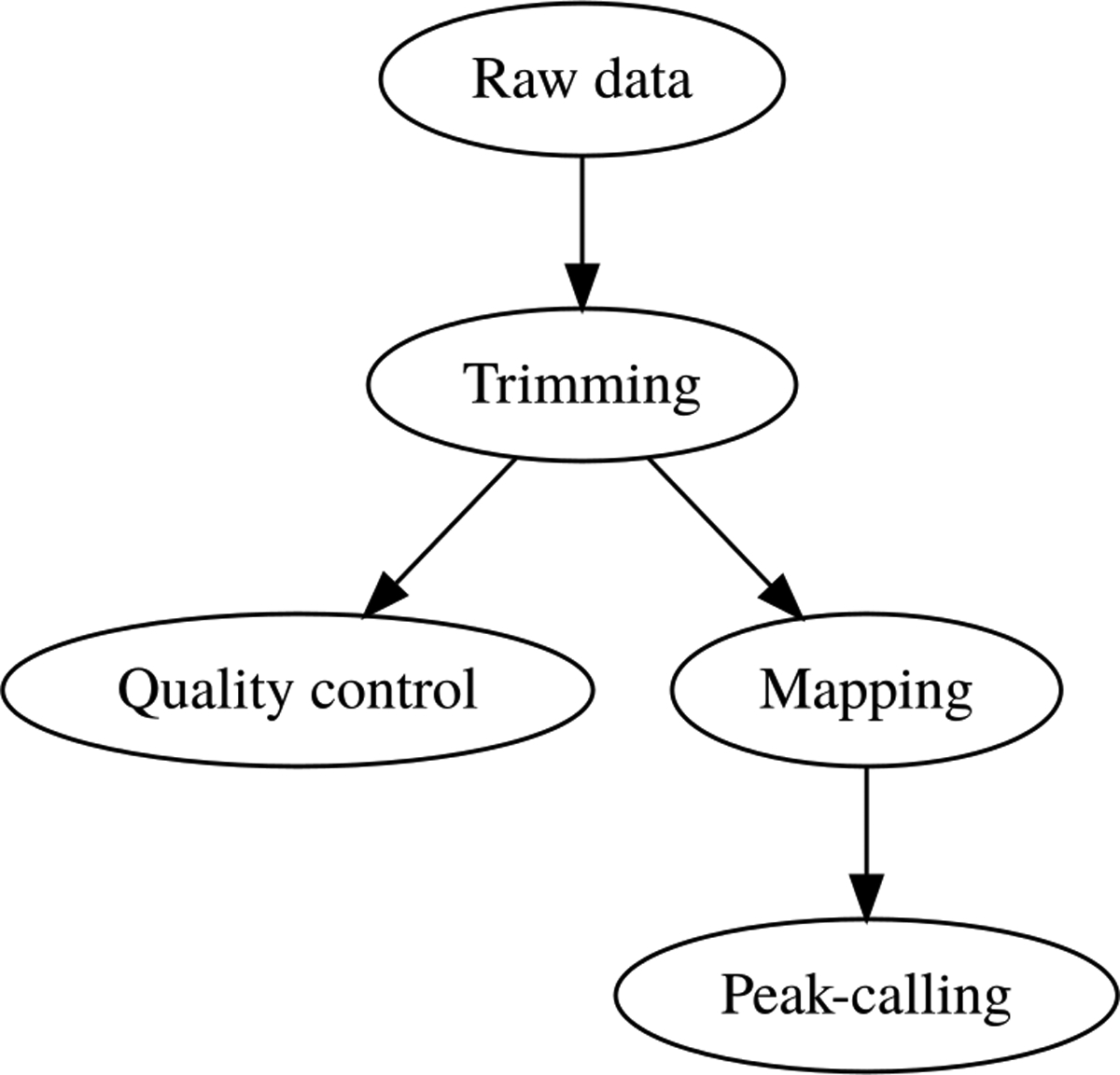
Schematic wiring of a basic workflow for ChIP-seq analysis.

The exploitation of the data by properly implemented bioinformatics workflows (comprehensive specification of the tools, their versions and selection of parameters) is crucial to ensure traceability and reproducibility of the results from the raw data. A workflow also enables to perform identical treatments on dozens of samples, using powerful computing infrastructures when necessary. Snakemake (Köster and Rahmann, 2012) is a software conceived for building such workflows. Based on the python language, it inherits concepts from GNU make (https://www.gnu.org/software/make): a workflow is defined by a set of rules, each defining an operation characterized by its inputs, outputs and parameters, and a list of target files to be generated through these operations.

SnakeChunks is a library of workflows using the Snakemake framework and designed for the analysis of ChIP-seq and RNA-seq data. It includes rules for the quality control of the sequencing reads, removal of adapters and trimming of low-quality bases, read mapping on a reference genome, peak-calling to detect local enrichment of reads resulting from the binding of a transcription factor, gene-wise quantification of RNAs, and differential gene expression analysis (Figure 2a).

Figure 2. Organization of the SnakeChunks library.

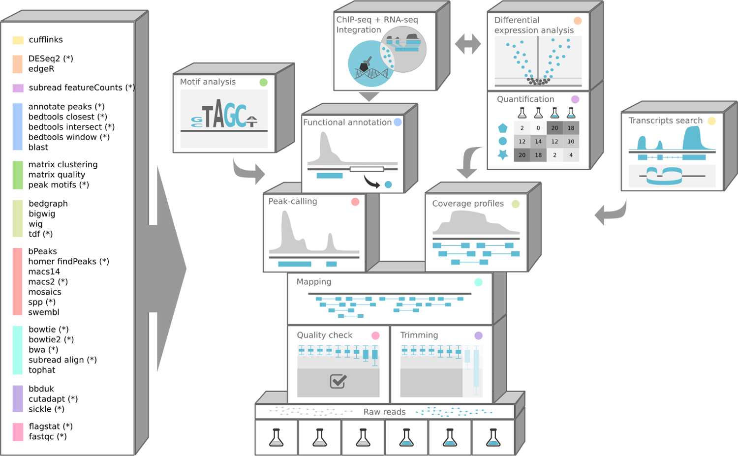
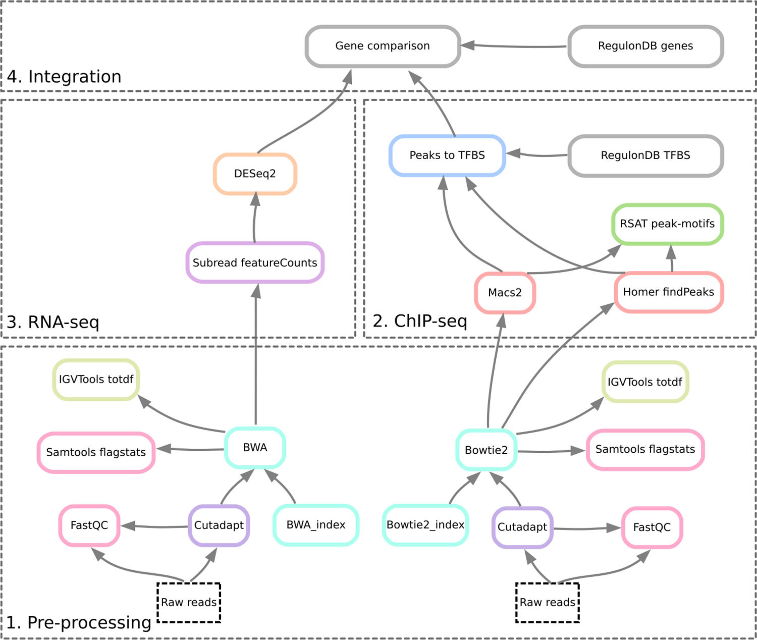
(a) Principle of the SnakeChunks library. The library is built around a set of snakemake rules that can be used as building blocks to build workflows in a modular way. Each rule allows to perform a given type of operation with a given tool. A given operation can be done with alternative tools, as denoted by the color code in list of rules (left side) and on the building bricks. The rules marked with an asterisk (*) are currently supported by conda. (b) Schematic flowchart of the workflows described in this protocol.

The SnakeChunks library has been used to analyse RNA-seq data from Mus musculus, Drosophila melanogaster, Saccharomyces cerevisiae, Glossina palpalis (Tsagmo et al. 2017) and Desulfovibri desulfuricans (Cadby et al., 2017) as well as ChIP-seq data from Arabidopsis thaliana (Castro et al. 2016). We illustrate here its use on combined RNA-seq and ChIP-seq data from Escherichia coli (Myers et al., 2013).

Since the description of the operon structure (Jacob and Monod, 1961), Escherichia coli K-12 has been a model organism of reference for the study of gene regulation, resulting in thousands of publications reporting information about around 200 of the total ~300 transcription factors (TFs) identified in its genome (Blattner et al., 1997; Pérez-Rueda and Collado-Vides, 2000). Detailed information about TFs, their binding sites, binding motifs, target genes and operons has been collected for three decades in RegulonDB, the database on transcriptional regulation in E.coli (Gama-Castro et al., 2016), by manual curation of publications based on low-throughput experiments. Yet, a lot of information remains to be discovered to reach a global comprehensive picture of the regulatory network in the best-characterized model organism. Next-Generation Sequencing (NGS) technologies enable the characterization of biological regulation at an unprecedented scale, and have been widely adopted by research communities. ChIP-seq gives insight into regulatory mechanisms by providing genome-wide binding locations for transcription factors, whereas RNA-seq informs about the functional implications of regulation by measuring the level of transcription of all genes in different conditions.

ChIP-seq publications initially focused on Human and metazoan models (Pubmed currently returns 1,600 ChIP-seq studies for Homo sapiens, and more than 2,000 for Mus musculus), and a surprisingly small number of factors were characterized by ChIP-seq in Escherichia coli (44 entries in Pubmed). However, systematic studies have been led to characterize 50 transcription factors of Mycobacterium tuberculosis (Galagan et al., 2013), and similar projects are on the way for other bacteria, including E. coli. The protocols described here address the foreseeable needs of microbiologists undertaking projects based on ChIP-seq, RNA-seq or the combination of both technologies to analyse bacterial regulation. Those are illustrated by a study case based on a genome-scale analysis of the FNR transcription factor (Myers et al., 2013), a DNA binding protein that regulates a large family of genes involved in cellular respiration and carbon metabolism during conditions of anaerobic cell growth.

This unit is organised in basic protocols as follows.

• Strategic planning: installation and configuration of the software environment (Conda environment, software tools, SnakeChunks library, reference genome).

• Basic protocol 1: Pre-processing, which includes quality control, trimming and mapping of the raw reads on the reference genome. This protocol is illustrated with the ChIP-seq study case but can be applied to RNA-seq data as well.

• Basic protocol 2: analysis of ChIP-seq data: peak-calling, assignation of peaks to genes, motif discovery, comparison between ChIP-seq peaks and sites annotated in RegulonDB.

• Basic protocol 3: analysis of RNA-seq data: preprocessing (as in Basic Protocol 1), transcript quantification (counts per gene), detection of differentially expressed genes (DEG).

• Basic protocol 4: integration of ChIP-seq and RNA-seq results: comparison between genes associated to the ChIP-seq peaks, DEG reported by transcriptome analysis, and experimentally-proven TF target genes annotated in RegulonDB. Visualisation of the results using a genome browser.

• Alternate protocol 1: running the RNA-seq workflow with the user-friendly graphical interface Sequanix.

• Supplementary protocol 1: customization of the parameters of the ChIP-seq workflow.

The basic protocols are conceived in a modular way (Figure 2b). In particular, ChIP-seq and RNA-seq analyses can be done separately.

NECESSARY RESOURCES

Computer resources

This protocol runs on any Unix system (Linux, Mac OS X). Memory and CPU requirements depend on the data volumes to be treated. The study cases have been tested on Ubuntu 14.04, 16.04 and 18.04 (4 CPUs, 16Gb RAM), Centos 6.6, and on Mac OSX High Sierra (4 CPU, 16Gb RAM).

The full protocol uses about 60Gb of disk space, including ~5Gb for the installation of the software environment (conda, libraries and tools), ~15Gb of downloaded raw reads (compressed fastq files, genome annotations), and ~40Gb for the intermediate and final result files.

The total processing time is ~12h for all the tasks, of which 45% is spent on the read mapping and 33% on the trimming of RNA-seq samples. This time might be further reduced by parallelizing some tasks on a multi-CPU server or cluster (on our 4-core configurations, the analyses were completed in ~3h).

Conda

Conda is an open source package and environment management system used to automate the installation of all software components required by the workflows. It greatly facilitates the installation of software tools from multiple sources on different Unix operating systems (Linux, Mac OS X). In addition, the installation and use of all the software tools inside a custom environment ensures their isolation from the hosting system and prevents potential clash with the existing tools and libraries.

Conda should be installed prior to the execution of the protocol. It comes in two different versions: Anaconda and Miniconda. We recommend installing Miniconda, which takes less disk space and allows one to install only the required software. Instructions can be found here: https://conda.io/docs/user-guide/install/index.html.

You should make sure that the folder containing the conda executable is added to your $PATH variable. This can be done automatically during the execution of the Miniconda installation script, or done later by adding the following command in your bash profile (file ~/.bash_profile).

export PATH=$PATH:~/miniconda3/bin/

You now need to log out and open a new terminal session in order for the path to be updated.

Other software

In the protocol we use the program tree to display the structure of folders and included file in the Unix terminal. This software is not properly speaking required for the analysis, but offers a convenient way to check the proper organisation of the files in the shell. Its installation can vary depending on the operating system or Linux distribution. Here are some examples of installation with some popular package management systems.

Linux Ubuntu: sudo apt-get install tree

Linux CentO: sudo yum install tree

Mac OS X : brew install tree

Note: in the following protocols, the instructions (courier font) should be typed or copy-pasted in a terminal.

STRATEGIC PLANNING

Configuration of the Conda environment

This section provides a succession of Unix commands that enable to configure conda, create a specific environment, install the required software (Snakemake and NGS tools), and download the reference genome and annotations (in our case, Escherichia coli K-12 MG1655, release 37).

1. Configure Conda.

       conda config --add channels r;
       conda config --add channels defaults;
       conda config --add channels conda-forge;
       conda config --add channels bioconda
   

   Note: it is important for these commands to be typed in the precise order indicated above, which defines the priorities for packages that would exist in several channels. Conda might issue warnings that can be ignored, when some of the channels are already present. We intently re-add these channels in order to place them in the right order of precedence.

2. Create an empty environment using python version 3.6.

       conda create --name snakechunks_env python=3.6
   

3. Activate the environment.

   Beware: this must be done for each new session of analysis.

       source activate snakechunks_env
   

   Check that the environment is active: the unix prompt is prepended by “(snakechunks_env)”

4. Install Snakemake and some required software tools in the conda environment: GNU make software, python panda library, and the Integrative Genome Viewer IGV.

       conda install make snakemake=5.1.4 igv=2.4.9 pandas=0.23.4
   

5. Define an environment variable with the directory for this analysis.

   Beware: this must be done for each new session of analysis (alternatively you can declare it in your bash profile).

       export ANALYSIS_DIR=$HOME/FNR_analysis
   

6. Create the analysis directory.

       mkdir -p $ANALYSIS_DIR
   

7. Set current working directory to the analysis directory.

   Beware: this must be done for each new session of analysis.

       cd $ANALYSIS_DIR
   

8. Download the SnakeChunks library from Github. We recommend keeping a copy of the library in the analysis directory to ensure consistency and reproducibility.

   Downloading the latest version of the SnakeChunks library can be done easily with the git command.

       git clone https://github.com/SnakeChunks/SnakeChunks.git
   

   Note: the SnakeChunks code will keep evolving with time. For the sake of backward compatibility, we froze the precise version of the library used at the moment of publishing this protocol. This version can be downloaded with the following command.

       wget --no-clobber \
          https://github.com/SnakeChunks/SnakeChunks/archive/4.1.3.tar.gz
       tar xvzf 4.1.3.tar.gz
       mv SnakeChunks-4.1.3 SnakeChunks
   

9. Download the reference genome of E.coli K-12 and its annotations.

       make -f SnakeChunks/examples/GSE41195/tutorial_material.mk \
         download_genome_data
   

10. Check the organisation of the files in the genome directory (Figure 3).

        tree -L 2
    

    Note The above steps describe how to setup the environment and needs to be executed only once, except for steps 3, 5 and 7, which are required for each working session for this project. If you log out of the terminal and want to start a new session later, you will have to reactivate the conda environment (step 3), redefine the environment variable for the analysis directory (step 5) and set it as current directory (step 7).

Figure 3.

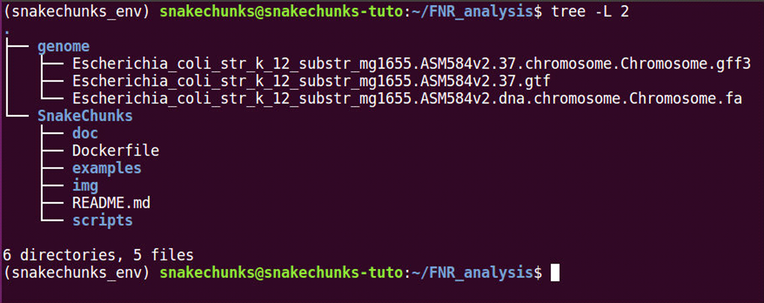
Checkpoint of the file organization after having completed the Strategic Planning section.

BASIC PROTOCOL 1: DATA PREPROCESSING AND READ MAPPING

Data preprocessing covers the first steps of the analysis, which are common to most NGS workflows. The goal is to make sure that the raw sequencing data is suitable for a proper bioinformatics analysis. This includes quality control of the sequenced reads, removal of the sequencing adapters, and trimming of the read extremities when needed. These operations are described more thoroughly in the Guidelines for Understanding Results section below.

We illustrate theses steps with a ChIP-seq dataset, but they can be applied similarly to RNA-seq data.

Once the reads are processed and filtered appropriately, a common operation to perform before ChIP-seq and RNA-seq analyses is to map the reads on a reference genome in order to identify their genomic location.

This protocol covers the following steps:

• Quality control of the reads using the program FastQC (Andrews, 2010);

• Removal of the adapters and trimming of the read extremities using cutadapt (Martin, 2011);

• Read mapping using the algorithm bowtie2 (Langmead et al., 2012).

Protocol steps—Step annotations

1. Download the ChIP-seq dataset from the GEO series GSE41195 (Myers et al., 2013).

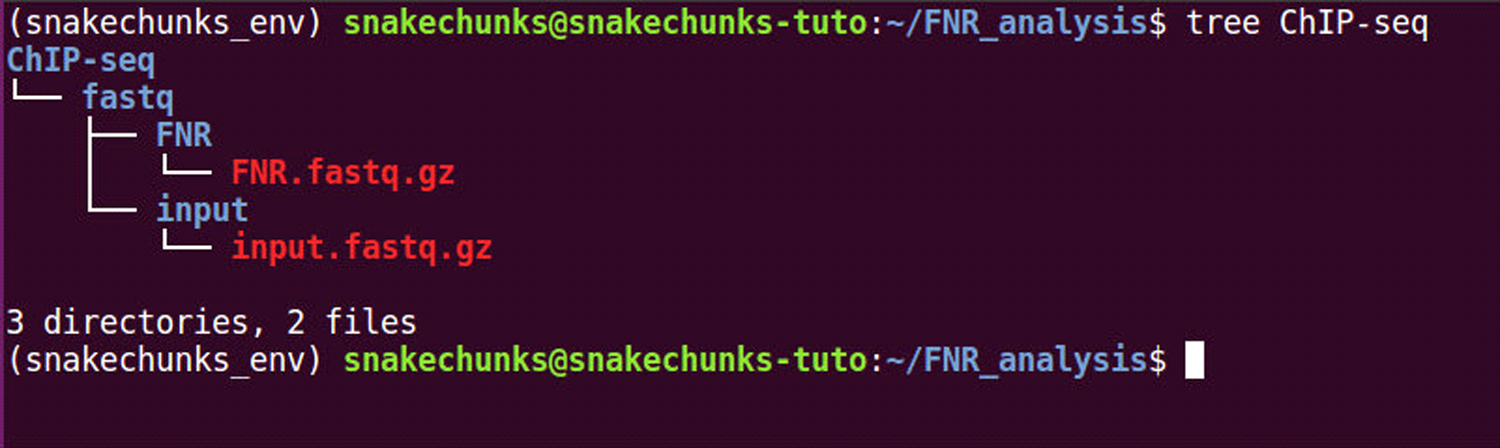
       make -f SnakeChunks/examples/GSE41195/tutorial_material.mk \
       download_chipseq_data
   

   This creates a subdirectory “ChIP-seq” in the analysis directory defined in the Strategic Planning section (Figure 4), with two fastq files corresponding to the FNR-chipped and to the control samples, respectively.

       tree ChIP-seq
   

2. Create a local copy of the metadata folder.

       make -f SnakeChunks/examples/GSE41195/tutorial_material.mk copy_metadata ;
       tree metadata
   

   This creates a local copy of the metadata folder, which contains files describing the samples, the analysis design, and the workflow configuration.

3. Run the workflow for quality control.

       snakemake -s SnakeChunks/scripts/snakefiles/workflows/quality_control.wf \
       --configfile metadata/config_ChIP-seq.yml --config trimming=““ -p --use-conda
   

   The command above runs a workflow using the snakemake command with the following specifications.

   • The wiring of the workflow is defined in the file quality_control.wf, specified with the option -s. Modifying this wiring requires some knowledge of the snakemake language, which is out of scope for this protocol (snakemake tutorials can be found in the Snakemake documentation: http://snakemake.readthedocs.io/en/stable/tutorial/tutorial.html).
   • The workflow invokes a series of tools, each of which can be tuned with different parameters. All the parameters of the workflow are specified in a yaml-formatted configuration file, specified with the option --configfile. The yaml format is human-readable and can be easily edited with a standard text editor (see section Support protocol 1 below).
   • The option --config is used in order to specify that trimming will not be performed during this run. It overrules the configuration defined in the configuration file above mentioned, which is to perform trimming automatically, as will be done in step 5.
   • The option -p tells snakemake to print out all the Unix commands that will be executed. This listing is very convenient to check that each command is called with the appropriate parameters, and to keep a trace of the full process between raw data and final results.
   • When the option --use-conda is used, Snakemake creates a separate virtual environment for each rule executed in the workflow, and installs the required tools and their dependencies in a rule-specific subfolder. This ensures compatibility between the different tools invoked. The process can take some time at the first invocation of a given environment, but is faster for subsequent uses of the same environment.
   • The workflow quality_control.wf produces quality reports using the FastQC tool (Andrews, 2010). This is an essential step to assess the quality of the samples, and plan the forthcoming steps of the analysis.
4. The presence of the two FastQC reports can be checked with the ls commands below.

       ls -l $ANALYSIS_DIR/ChIP-seq/fastq/FNR1/FNR1_fastq.gz_qc/FNR1_fastqc.html;
       ls -l $ANALYSIS_DIR/ChIP-seq/fastq/input1/input1_fastq.gz_qc/input1_fastqc.html
   

   These files can be opened with a Web browser. Insights about these reports can be found in the Guidelines for Understanding Results section below.

5. Run the quality control workflow again, using the software cutadapt, which performs both trimming of the reads and adapter removal.

       snakemake -s SnakeChunks/scripts/snakefiles/workflows/quality_control.wf \
          --configfile metadata/config_ChIP-seq.yml -p --use-conda
   

   This time, the workflow will run cutadapt, as defined in the configuration file, before doing a new FastQC check. Note that SnakeChunks allows one to specify several tools for a same step, in order to compare the results. An overview of the possibilities is proposed in the Support Protocol 1 section.

6. The presence of FastQC reports can be checked with the ls commands below.

       ls -l \
       $ANALYSIS_DIR/ChIP-seq/fastq/FNR1/FNR1_cutadapt_fastq.gz_qc/FNR1_cutadapt_fastqc.html;
       ls -l \
       $ANALYSIS_DIR/ChIP-seq/fastq/input1/input1_cutadapt_fastq.gz_qc/input1_cutadapt_fastqc.html
   

   Open the new FastQC reports with a Web browser. The reports show the improvement of the quality of the reads, as well as the absence of overrepresented sequences corresponding to adapters. This is further discussed in the Guidelines for Understanding Results section below.

7. Run the read mapping workflow.

       snakemake -s SnakeChunks/scripts/snakefiles/workflows/mapping.wf \
          --configfile metadata/config_ChIP-seq.yml -p --use-conda -j 2
   

   This workflow essentially performs two operations: read mapping and genome coverage.

   We added the option -j 2, which permits snakemake to parallelize the processing, with a maximum of 2 simultaneous jobs. Since the mapping step can be time-consuming, it it recommended to run it in parallel for the different samples. This option should be adapted to the number of cores of your system. For example, if you analyse a large number of files on a cluster, you could increase the number of simultaneous jobs to 40 or even more (this has to be negotiated with the system administrator).

   More information about the mapping results can be found in the Guidelines for Understanding Results section.

8. Check the content of the files containing statistics of the mapping from the shell.

       cat \
          $ANALYSIS_DIR/ChIP-seq/results/samples/FNR1/FNR1_cutadapt_bowtie2_bam_stats.txt;
       cat \
          $ANALYSIS_DIR/ChIP-seq/results/samples/input1/input1_cutadapt_bowtie2_bam_stats.txt
   

   These files, generated by the program samtools flagstat, display basics statistics for the mapping. As can be seen on Figures 5a and 5b, both samples have a very high mapping rate, which proves again that the sequencing data is of good quality, and that we are going to dispose of a high quantity of data to perform the ChIP-seq analysis.

Figure 4.

File organization of the ChIP-seq samples, before running the analyses.

Figure 5.

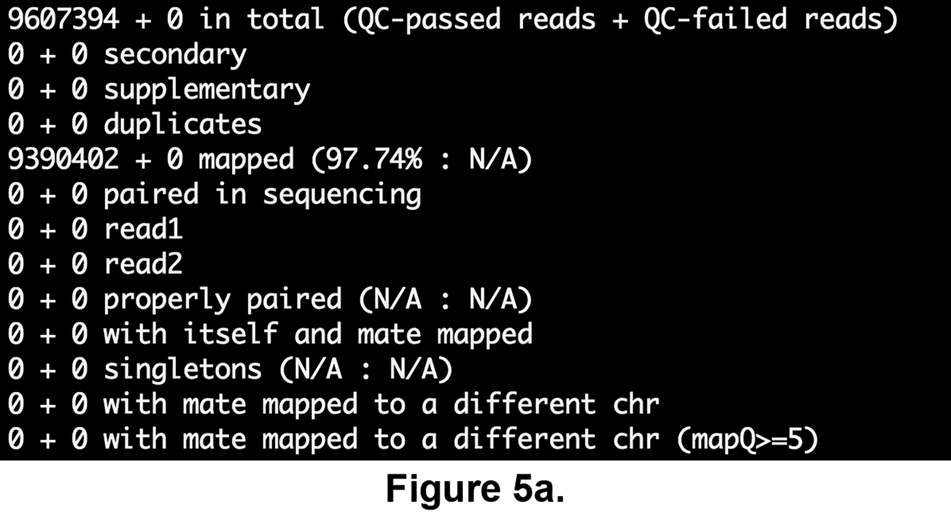
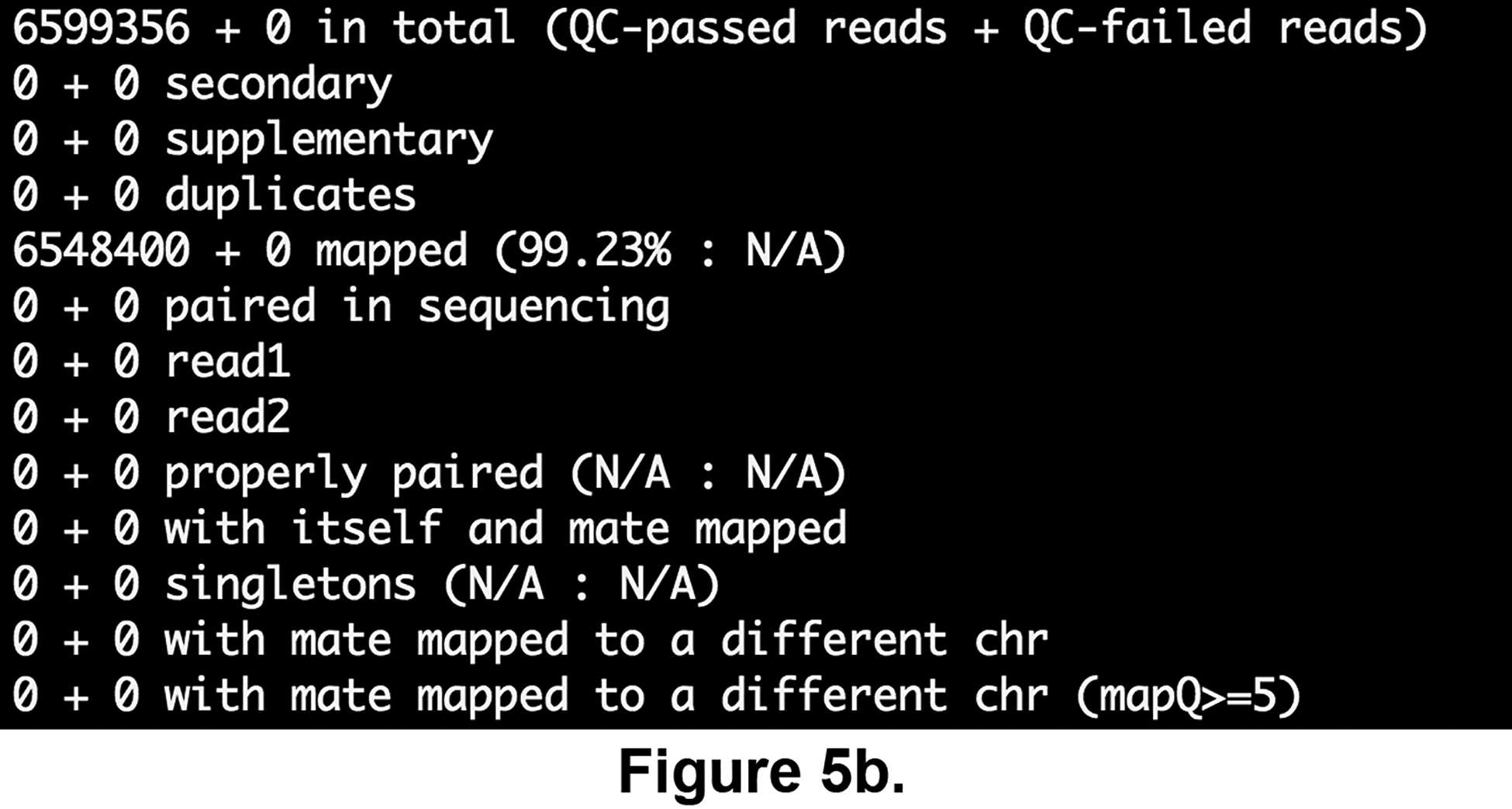
Read mapping statistics computed using the samtools flagstats software for the FNR ChIP-seq sample (a) and genomic input (b), respectively.

BASIC PROTOCOL 2: ChIP-seq

ChIP-seq (Johnson et al., 2007; Robertson et al., 2007) is a technology that allows for the characterization of DNA binding at a genome scale. The experiment includes the following steps: cross-linking DNA and the bound proteins with a fixative agent, breaking DNA into random fragments by ultrasonication, immunoprecipitating a transcription factor of interest together with its cross-linked DNA, unlinking these DNA fragments, amplifying them by PCR and sequencing them with massively parallel sequencing technologies. The raw sequences (“reads”) are then mapped onto a reference genome, and putative binding regions denoted as “peaks”, which are covered with a high number of reads and usually extend over a few hundred base pairs. These peaks can then be used to search for precise transcription factor binding sites (TFBS), which can then be associated to a nearby gene to infer the potential TF target genes.

A critical step of a ChIP-seq data analysis is peak-calling, which consists in detecting these genomic regions with a higher density of mapped reads than would be expected by chance. The choice of a peak-calling algorithm and the tuning of its parameters can drastically affect the number of returned peaks and their sizes. In order to identify reliable peaks and avoid false positives, it is important to use control samples (see Commentary section for more details). Peak-callers also have some parameters enabling to tune the rate of false positives by imposing more or less stringent thresholds on peak scores, in order to optimise the tradeoff between sensitivity (the proportion of actual binding regions detected) and specificity (the capability to reject non-binding regions).

Here, we are going to compare two samples (Table 1): a test sample resulting from the immunoprecipitation of the FNR transcription factor, and a genomic input.

Table 1. Description of the ChIP-seq samples.

Column headers indicate their contents. The columns ID and Condition are mandatory for the proper use of the workflow. Additional columns can be added at will to document samples.

ID	Condition	GSM identifier	SRR identifier
FNR1	FNR	GSM1010220	SRR576934
input1	input	GSM1010224	SRR576938

While many publications rely on the Macs2 peak-caller (Feng et al., 2011), generally used with its default parameters, there are actually a variety of tools that can be used and customized in different ways (Pepke et al., 2009). SnakeChunks currently supports 7 of them, in a completely interchangeable way (Figure 2a). Here we are going to demonstrate how to use two of them: Homer (Heinz et al., 2010) and Macs2. Those peak-callers are two of the most widely used, maintained and up-to-date programs, and are also supported by conda.

The main operations performed by the workflow are the following:

• Peak-calling using Homer and Macs2 (Heinz et al., 2010; Feng et al., 2011);

• Motif discovery by remote invocation of the tool peak-motifs (Thomas-Chollier et al., 2012) from the RSAT software suite (Nguyen et al., 2018) via its Web services interface. RSAT peak-motifs also compares discovered motifs with the TF binding motifs annotated in RegulonDB;

• Comparison between ChIP-seq peaks and known TFBS listed in the RegulonDB database (Gama-Castro et al., 2016);

• Assignation of genes to the peaks with the tool annotate peaks from the Homer suite;

• Gene comparison: comparison between genes associated to peaks and TF target genes (as annotated in RegulonDB).

Protocol steps—Step annotations

1. Run the ChIP-seq workflow.

       snakemake \
          -s SnakeChunks/scripts/snakefiles/workflows/ChIP-seq_RegulonDB.wf\
          --configfile metadata/config_ChIP-seq.yml -p --use-conda -j 2
   

2. The output files can be found here.

   1. Peaks. Since these files are quite large, we use the less unix command to display them page by page (press enter to move one page forward). After having inspected a few pages, type “q” to quit the less program.

          less \
          $ANALYSIS_DIR/ChIP-seq/results/peaks/FNR1_vs_input1/homer/FNR1_vs_input1_cutadapt_bowtie2_homer.bed ;
          less \
          $ANALYSIS_DIR/ChIP-seq/results/peaks/FNR1_vs_input1/macs2/FNR1_vs_input1_cutadapt_bowtie2_macs2.bed
      

   2. Motifs discovered with RSAT in the peaks. Check that the html files produced by peak-motifs are at the expected place.

      ls -l \
      $ANALYSIS_DIR/ChIP-seq/results/peaks/FNR1_vs_input1/homer/peak-motifs/FNR1_vs_input1_cutadapt_bowtie2_homer_peak-motifs/peak-motifs_synthesis.html ;
      ls -l \
      $ANALYSIS_DIR/ChIP-seq/results/peaks/FNR1_vs_input1/macs2/peak-motifs/FNR1_vs_input1_cutadapt_bowtie2_macs2_peak-motifs/peak-motifs_synthesis.html
      

      Open the peak-motifs reports with a Web browser. The results of this workflow are further described in the Guidelines for Understanding Results section below.

BASIC PROTOCOL 3: RNA-seq

RNA-seq technology, or whole transcriptome shotgun sequencing, reveals the presence or absence of RNA from a given sample, at a given moment in time, and also quantifies them if needed. It consists of extracting the total RNA from a cell and filtering out genomic DNA using a deoxyribonuclease (DNase). The RNA is then reverse-transcribed to cDNA, which can either be mapped onto a genome of reference, or assembled de novo. Subsequent possibilities of analysis include the quantification of gene expression, the identification of alternative transcripts, or single-nucleotide variation discovery.

In this protocol, we will use an RNA-seq experiment published by Myers and collaborators (2013) as a case study, where the transcriptome of E. coli K-12 was measured in two samples from wild type (WT) and from a mutant strain where the FNR transcription factor activity is inhibited (Lazazzera et al., 1993). In order to perform reliable RNA-seq analyses, it is crucial to dispose of biological replicates (see Commentary section). This dataset includes two replicates per genotype (Table 3). Our goal will be to identify genes that are differentially expressed between the FNR mutant (defined as test condition in Table 4) and the WT (reference condition).

Table 3. Description of the RNA-seq samples.

Column headers indicate their contents. The columns ID and Condition are mandatory for the proper use of the workflow. Additional columns can be added at will to document samples.

ID	Condition	GSM identifier	SRR identifier
WT1	WT	GSM1010244	SRR5344681
WT2	WT	GSM1010245	SRR5344682
dFNR1	FNR	GSM1010246	SRR5344683
dFNR2	FNR	GSM1010247	SRR5344684

Table 4. Experimental design of the RNA-seq analysis.

The design file can contain one or several rows, each describing a pair of conditions to be compared. The Test and Reference conditions must correspond to the values in the “Condition” column of the sample description table.

Test	Reference
FNR	WT

This workflow performs the following steps.

• Quality control and trimming of the reads (for further detail, see Basic Protocol 1);

• Mapping onto a genome of reference using the algorithm BWA (Li et al., 2009) (for further detail, see Basic Protocol 1).

• Quantification of transcripts per gene with featureCounts from the Subread package (Liao et al., 2014).

• Detection of differentially expressed genes with DESeq2 (Love et al., 2014) and edgeR (Robinson et al., 2010).

• Automatic generation of a report summarizing the results.

Protocol steps—Step annotations

1. Copy the example metadata from the SnakeChunks library (can be skipped if already done in Basic protocol 1, step 2), and check the content of the metadata folder.

       make -f SnakeChunks/examples/GSE41195/tutorial_material.mk copy_metadata;
       tree metadata
   

2. Download RNA-seq data.

   make -f SnakeChunks/examples/GSE41195/tutorial_material.mk download_rnaseq_data
   

   This creates a subdirectory “RNA-seq” in the analysis directory defined in the Strategic Planning section (Figure 6), and downloads the raw data. Beware: during our tests, the download takes approximately 8 minutes per sample. Since the analysis requires 8 files, this download step can take up to a few hours depending on your connection speed. After the command has been completed, check the organization of the downloaded files.

   tree -C RNA-seq
   

   You should now see 4 directories (one per sample) each containing two files with extension .fastq.gz (there is one file per sequencing end).

3. Run the RNA-seq analysis workflow.

       snakemake -s SnakeChunks/scripts/snakefiles/workflows/RNA-seq_complete.wf \
       --configfile metadata/config_RNA-seq.yml -p --use-conda -j 4
   

   Note: here we use the option -j 4 in order to parallelize the treatment of the four samples, which is time-consuming.

4. Check the organisation of the result files in the RNA-seq folder, with a folder depth limit of 3.

       tree -C -L 3 RNA-seq
   

5. The results of the differential expression analysis performed by this workflow are summarized in an automatically generated HTML report, which can be opened using a web navigator.

       RNA-seq/results/diffexpr/cutadapt_bwa_featureCounts_rna-seq_deg_report.html
   

   The elements of this report are further described in the Guidelines for Understanding Results section below.

6. Optionally, we can already check the content of the main result files, which can be found here.

   ls -l RNA-seq/results/diffexpr
   

   This folder contains a table with the counts of reads per gene

   less RNA-seq/results/diffexpr/cutadapt_bwa_featureCounts_all.tsv
   

   and a subfolder with the differential analysis results produced by edgeR, DESeq2, and the combination of them.

   ls -l RNA-seq/results/diffexpr/FNR_vs_WT
   

   It also contains two tables with the differential analysis statistics returned by DESeq2 and edgeR, respectively.

   less \
   RNA-seq/results/diffexpr/FNR_vs_WT/cutadapt_bwa_featureCounts_FNR_vs_WT_DESeq2.tsv;
   less \
   RNA-seq/results/diffexpr/FNR_vs_WT/cutadapt_bwa_featureCounts_FNR_vs_WT_edgeR_TMM.tsv
   

   The subset of differentially expressed genes (those declared positive because they pass the significance threshold) are exported in an additional file.

   less \
   RNA-seq/results/diffexpr/FNR_vs_WT/cutadapt_bwa_featureCounts_FNR_vs_WT_DEG_table.tsv
   

   Note: In the tutorial, we retain the union of genes called positive by either DESeq2 or edgeR but the combination rule can be tuned in the yaml configuration file.

7. We can count the rows of this file to get an idea of the number of differentially expressed genes (after having subtracted one for the header line).

   wc -l \
   RNA-seq/results/diffexpr/FNR_vs_WT/cutadapt_bwa_featureCounts_FNR_vs_WT_DEG_table.tsv\
    | awk ‘{print $1 −1}’
   

Figure 6.

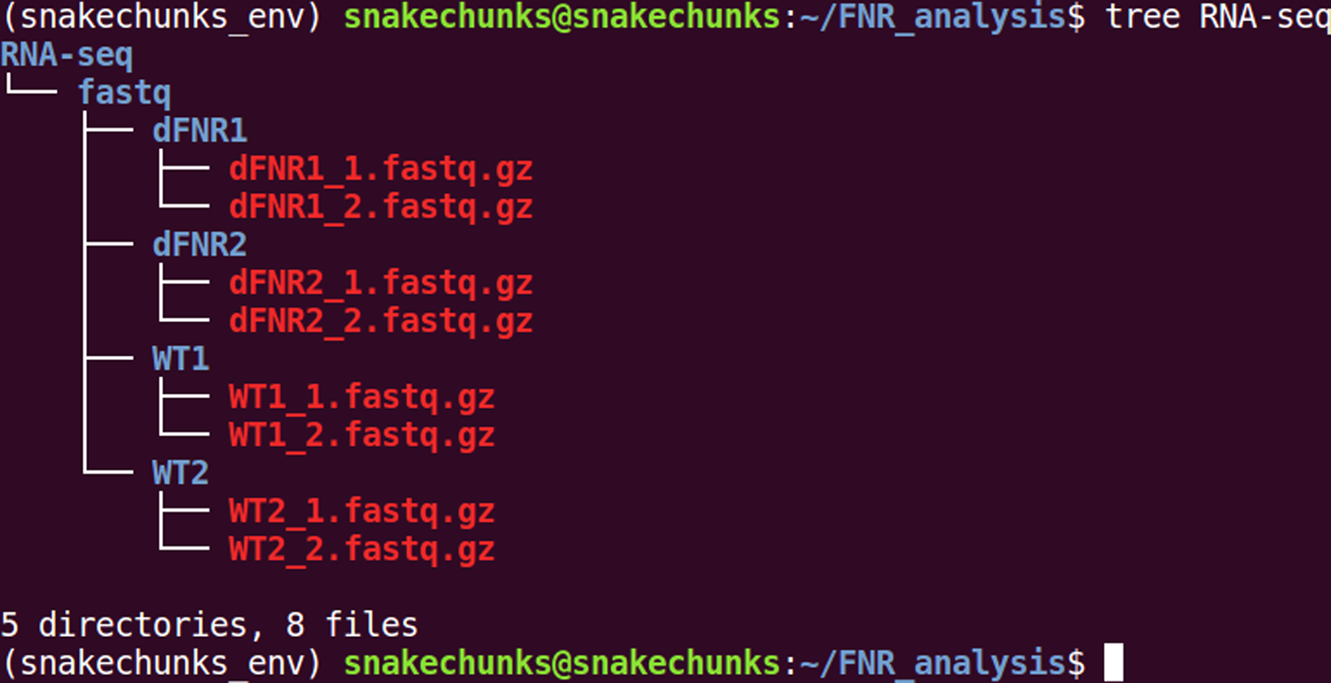
File organization of the RNA-seq samples, before running the analyses.

BASIC PROTOCOL 4: INTEGRATION

We have seen in Basic Protocol 2 that a ChIP-seq experiment followed by peak-calling enables to identify genomic binding locations for a given transcription factor. In Basic Protocol 3, we analysed results of an RNA-seq experiment to identify genes differentially expressed between two conditions (wild-type versus FNR mutant).

In this section, we show how to combine the results of those two types of experiments in order to unravel the links between genome binding data (ChIP-seq) and differential expression data (RNA-seq). This allows to detect direct target genes of a factor, i.e. genes whose transcription level is affected in the mutant, and whose upstream region contains a binding peak, but also indirect regulation (absence of a binding peak but effect on the expression of a gene), or binding of the FNR transcription factor without detected effect on the level of transcription of the associated genes. We also compare the NGS results with the list of FNR target genes annotated in the RegulonDB database (Gama-Castro et al., 2016).

1. Run integration workflow.

       snakemake -p \
         -s SnakeChunks/scripts/snakefiles/workflows/integration_ChIP_RNA.wf \
         --configfile metadata/config_integration.yml --use-conda
   

2. Check the first lines of the table summarizing the results per gene.

   less $ANALYSIS_DIR/integration/ChIP-RNA-regulons_gene_table.tsv
   

   For a better readability, we recommend to open this table with a spreadsheet software (Office Calc, Excel, …). This table contains annotations for all genes known in E.coli K-12, as well as indication of whether they are associated to FNR binding (ChIP-seq column), whether their transcription is affected by FNR (RNA-seq column), and whether they have been previously demonstrated to be regulated by FNR (FNR_regulon column).

3. Launch the Integrative Genome Browser (IGV) (Robinson et al., 2011; Thorvaldsdóttir et al., 2013).

   On Linux operating systems: igv

   Mac OS X : open the IGV in the Applications folder

4. Click on menu File, select Open session… and select the session file metadata/igv_session.xml in the FNR analysis directory.

   This will load an IGV session with our selection of relevant tracks for the interpretation of ChIP-seq and RNA-seq results, which will be further discussed in section “Guidelines for understanding results” below.

ALTERNATE PROTOCOL 1: RUNNING THE WORKFLOW WITH THE USER-FRIENDLY INTERFACE SEQUANIX

Sequanix (Desvillechabrol et al., 2018) is a graphical user interface (GUI) based on PyQt, developed in order to facilitate the execution of NGS Snakemake pipelines. It was originally developed to run workflows included in the Sequana project (http://sequana.readthedocs.io), but can also handle any Snakemake pipeline. Thanks to the graphical interface, the parameters can be customized easily and the workflows can be run without using any command line.

Here, we are going to demonstrate the execution of the RNA-seq workflow (see Basic Protocol 3) using this interface.

Necessary Resources

1. If not already done, create and activate a conda environment following the Strategic Planning section, steps 1–10.

2. Install Sequana.

       conda install -c bioconda sequana=0.7.1
   

3. If not already done, download the RNA-seq dataset following the Basic Protocol 3, step 1–2, in order to install the metadata and download RNA-seq raw reads.

Protocol steps—Step annotations

1. Launch sequanix.

       sequanix
   

2. In the top of the sequanix window, select the tab Generic pipelines.

3. Under the Snakefile tab, fetch the workflow file RNA-seq_complete.wf in the directory SnakeChunks/scripts/snakefiles/workflows.

4. Under the Config file tab, fetch the configuration file config_RNA-seq.yml in the directory metadata.

5. Under the Working directory tab, select the directory you defined above as $ANALYSIS_DIR (Strategic Planning, step 5) (Figure 7a.).

6. In the menu of the application, select Options > Snakemake options … > General, and type “--use-conda” in the bottom box “other options”, then press OK.

7. In the sequanix main window, press Save.

8. Press Show pipeline to check everything looks fine (Figure 7b.).

9. Press Run.

   Note: if you have followed Basic protocol 3, the Run button should not start any new analysis, because snakemake detects that the result files are already there. If not, sequanix will run the workflow just like in the terminal.

Figure 7. Sequanix graphical user interface.

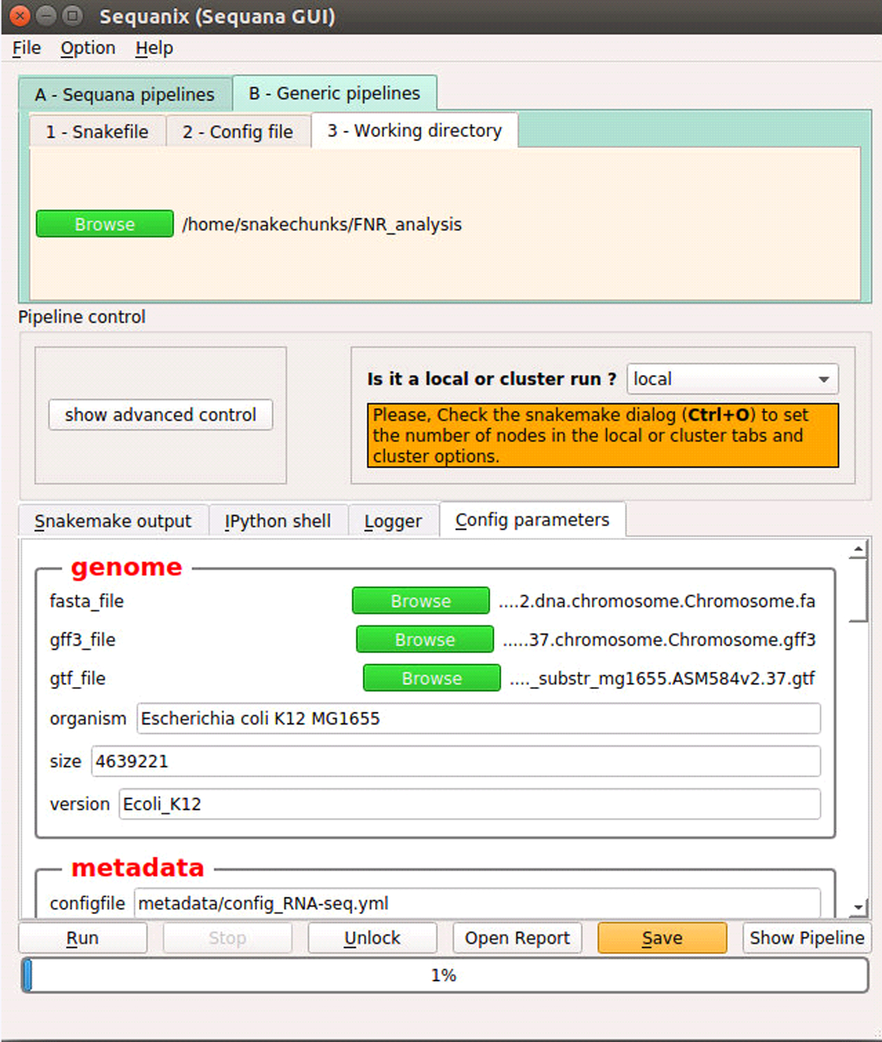
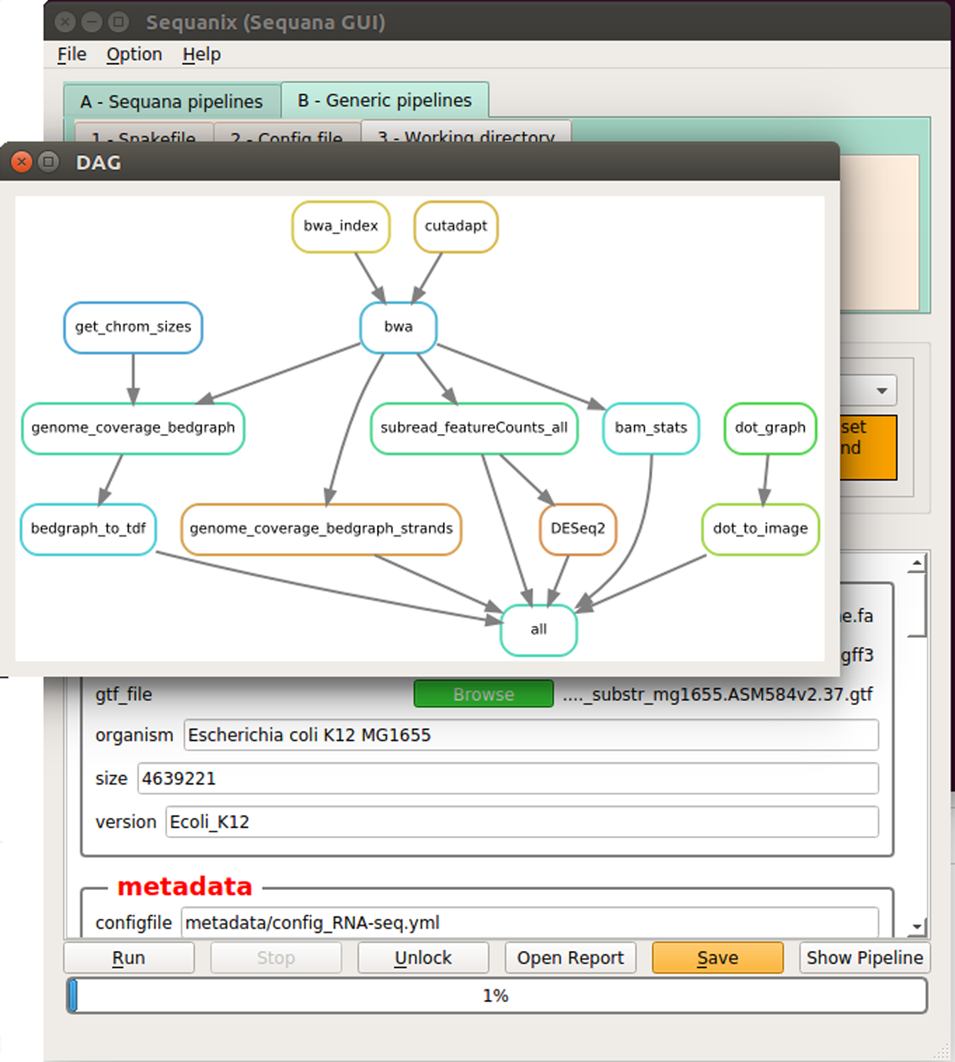
(a) Configuration the workflow parameters. (b) Display of workflow wiring. The diagram shows the directed acyclic graph (DAG) of rules automatically generated by snakemake.

SUPPORT PROTOCOL 1: CUSTOMIZATION OF THE PARAMETERS

Each workflow available in SnakeChunks requires three basic files in order to specify the input data files and all the parameters of an analysis. These files have been placed in a directory named “metadata”. We explain hereby how to adapt the ChIP-seq metadata files, but the same principle applies to the RNA-seq and integration workflows. The ChIP-seq workflow runs using 3 metadata files:

1. Sample file: samples_ChIP-seq.tab,

2. Design file: design_ChIP-seq.tab

3. Workflow and tool parameters: config_ChIP-seq.yml (Figure 8a).

Figure 8. Yaml-formatted configuration file for the ChIP-seq workflow.

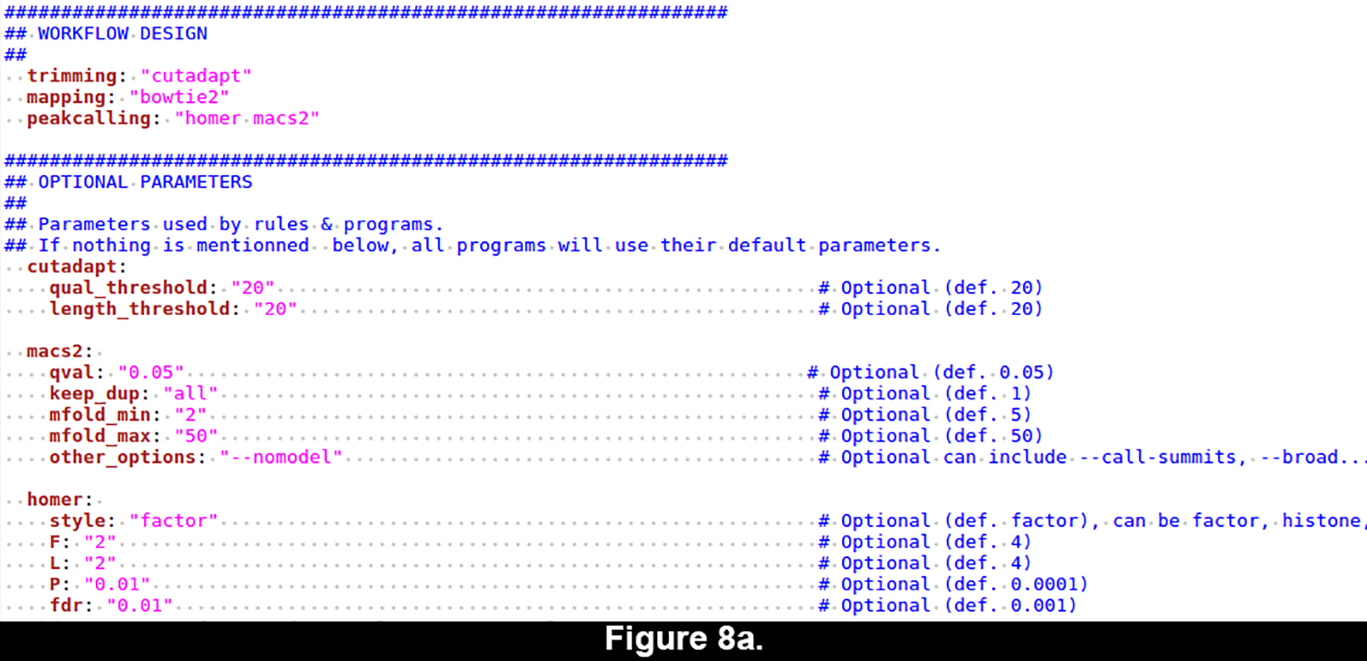
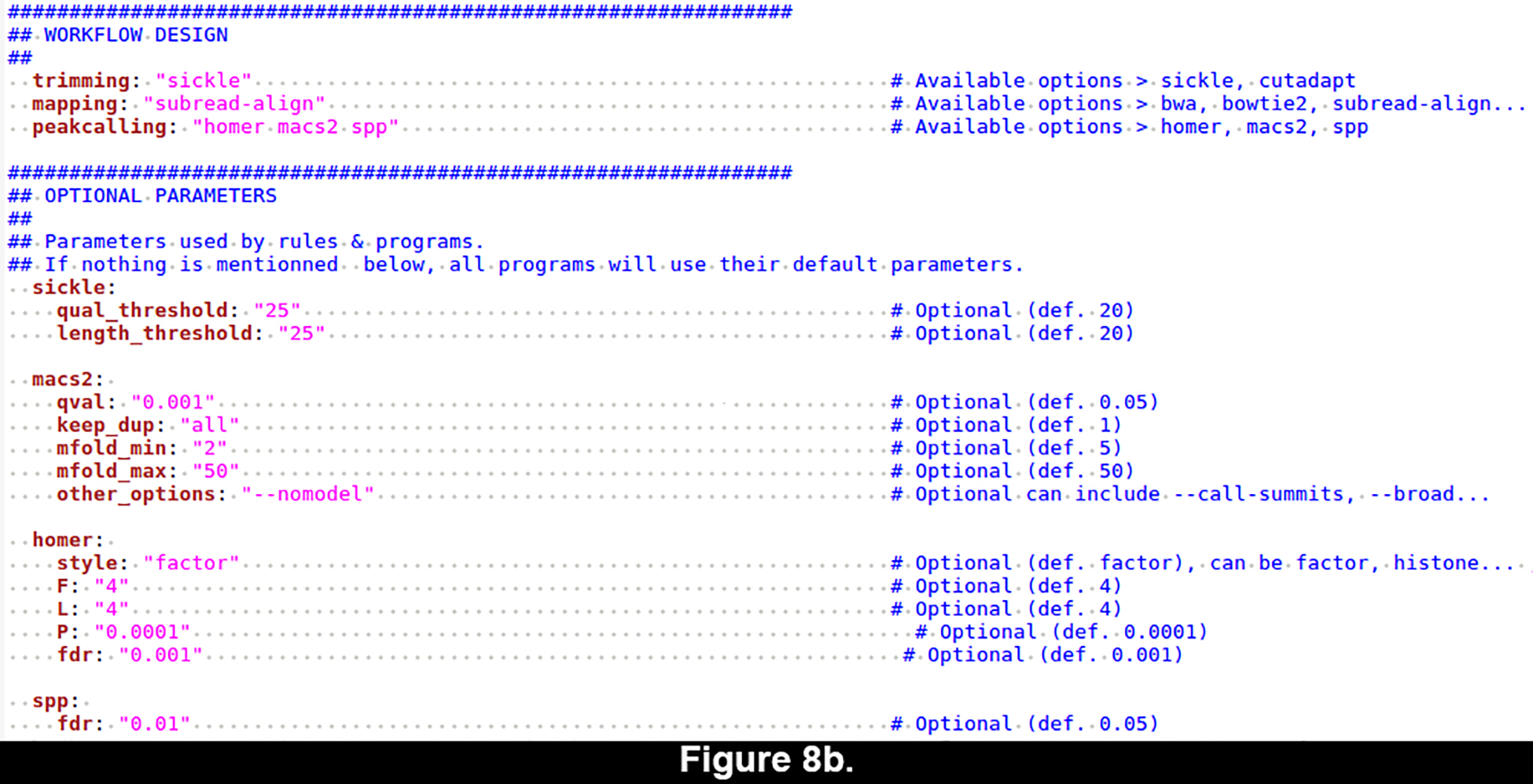
The yaml format enables to specify all the parameters of a workflow in a structured way whilst being human-readable and easily editable. (a) Default configuration. (b) Customized configuration.

The sample file (Table 1) describes each sample to be analysed (one row per sample), with two mandatory columns (ID and condition), and optional columns for complementary information such as GSM identifiers, etc. Here, we have two samples: one ChIP-ped with FNR, and a control sample labelled “input” following the ChIP-seq convention.

The design file (Table 2) defines the samples to be compared in order to perform peak-calling. Here, we are going to perform peak-calling of the ChIP sample, using the input sample as a background control. For RNA-seq, the design defines the conditions to be compared.

Table 2.

Experimental design of the ChIP-seq dataset.

Control	Treatment
input1	FNR1

The configuration file (Figure 8a) is specific to the workflow to be run. It contains three main parts: (1) general information about the genome of reference, the metadata file and the file organization; (2) general design of the workflow, such as the steps to be performed (trimming, mapping, peak-calling, annotation) and the tools to be used at each step; (3) an optional section enabling to customize the parameters used for each tool (if not specified, their default parameters are used).

In this part of the unit, we explain how to edit the configuration file in order to generate alternative results, using different tools and parameters.

Note: be aware that performing alternative trimming and/or mapping can require additional disk space, since FASTQ files (raw reads, trimmed reads) and BAM files (aligned reads) are very space-consuming. In the following protocol it requires about 2Go of disk space, but it can go up to tens of gigabases in the case of bigger raw files, like the RNA-seq files analysed in Basic Protocol 3.

Protocol steps—Step annotations

1. Create a copy of the ChIP-seq config file

       cd $ANALYSIS_DIR; \
       cp metadata/config_ChIP-seq.yml metadata/config_ChIP-seq_custom.yml
   

   Note: alternatively, you can avoid the manual edition of parameters by copying the ready-to-use customized configuration file provided in the distribution. For this, run the following command and skip the next step

   cp metadata/config_ChIP-seq_advanced.yml metadata/config_ChIP-seq_custom.yml
   

2. With a text editor, make the following changes to your custom configuration file (metadata/config_ChIP-seq_custom.yml).

   1. Change the trimming software from cutadapt to sickle.
   2. Change the mapping software from bowtie2 to subread-align.
   3. Add the spp peak-caller to Homer and Macs2.
   4. Customize spp, Homer and Macs2 parameters in the third section, according to the values shown in Figure 8b.
3. Run the commands below, which correspond to steps 1.5, 1.7 and 2.1 adapted to use the custom configuration file.

       snakemake \
          -s SnakeChunks/scripts/snakefiles/workflows/quality_control.wf \
          --configfile metadata/config_ChIP-seq_custom.yml -p --use-conda -j 2;
       snakemake \
          -s SnakeChunks/scripts/snakefiles/workflows/mapping.wf \
          --configfile metadata/config_ChIP-seq_custom.yml -p --use-conda -j 2;
       snakemake \
          -s SnakeChunks/scripts/snakefiles/workflows/ChIP-seq_RegulonDB.wf \
          --configfile metadata/config_ChIP-seq_custom.yml -p --use-conda -j 2
   

4. Visualize the differences in IGV: load a session as in Basic protocol 4 (integration), steps 3 and 4.

5. Click on menu File, select Load from File… and select the following peak files:

   $ANALYSIS_DIR/ChIP-seq/results_advanced/peaks/FNR1_vs_input1/spp/FNR1_vs_input1_sickle_subread-align_spp.bed
   $ANALYSIS_DIR/ChIP-seq/results_advanced/peaks/FNR1_vs_input1/homer/FNR1_vs_input1_sickle_subread-align_homer.bed
   $ANALYSIS_DIR/ChIP-seq/results_advanced/peaks/FNR1_vs_input1/macs2/FNR1_vs_input1_sickle_subread-align_macs2.bed
   

   Note: by running the command ‘wc -l’ on these files, you can note the influence of the choice of peak-caller, as well as it parameters.

GUIDELINES FOR UNDERSTANDING RESULTS

Data preprocessing and read mapping (Basic Protocol 1)

Quality control

For each sample, FastQC produces a box plot presenting per base sequence quality. A common phenomenon in high-throughput sequencing is the decrease of the sequence quality at the 3’ end of the reads. This can indeed be observed for the input sample (Figure 9). A low quality of the reads can reduce the percentage of mapped reads on the reference genome. To avoid this, we recommend sequence trimming in order to remove low-quality read extremities.

Figure 9. Quality report of the FNR1 ChIP-seq raw reads before trimming.

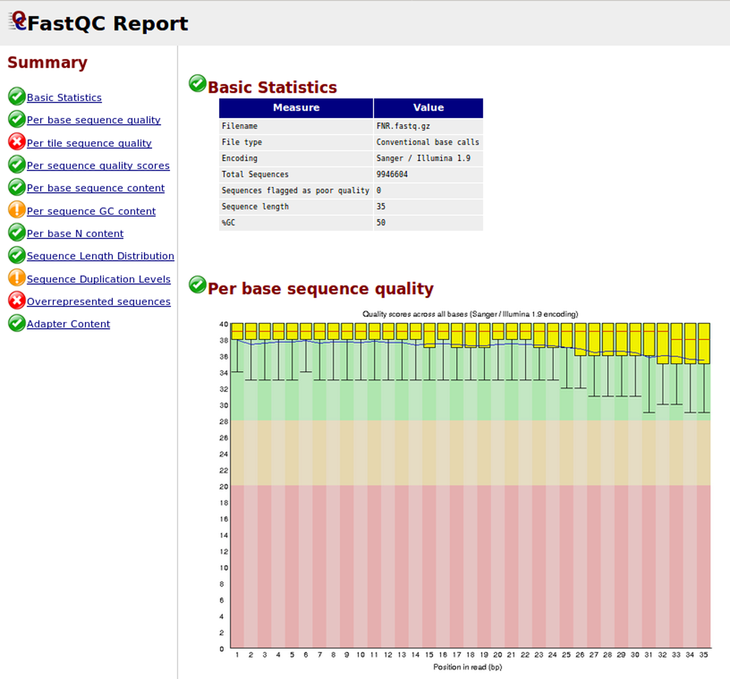
The abcsissa (columns) corresponds to nucleotide positions along the mapped reads, the ordinate indicates read quality scores. For each position, statistics are summarized for all the reads of a library: median (red line), interquartile range (yellow box), and quality range (vertical line). Background colors indicate an arbitrary subdivision of quality scores, from red (insufficient) to green (good).

Another interesting category of information in FastQC reports is the sequence duplication levels. The graph outlines read sequences found with an excessive number of copies, which may diagnose an effect of PCR amplification due to a poor complexity of the DNA library. Note that duplication is often interpreted in the context where the sequence library is much smaller than the genome size (typically ~50M reads for a ~3Gb Mammalian genome), so that reads resulting from a random sampling are not expected to fall on exactly the same genomic position. However, when studying bacterial regulation, library sizes can exceed genome size (typically 4Mb) so that multiple matches are expected along the whole genome. Another section of the FastQC report provides statistics about overrepresented sequences. Before removal of the adapters by cutadapt (Basic Protocol 1, step 5), Illumina adapters represent respectively 0.5% and 2.6% of the total number of reads of FNR1 and input1 samples. After using cutadapt, these sequences are gone (Basic Protocol 1, step 6). Detailed information for the interpretation of read quality is provided on the FastQC Web site (http://www.bioinformatics.babraham.ac.uk/projects/fastqc/).

Read mapping

Using the bowtie2 algorithm, the trimmed reads in FASTQ format are aligned onto a genome of reference, downloaded in the Strategic Planning section of this unit. In our case, the reference is Escherichia coli K-12. The result of the alignment comes in BAM format that keeps all the information from the fastq files about read sequences and quality, but adds their putative position in the reference genome.

Genome coverage

Genome coverage files enable to visualize the mapped reads in a condensed way, by showing the number of reads overlapping each position on each strand of the reference genome (Figure 10a, pink, grey and jade tracks in the middle panel) or their sum on both strands (purple track). Coverage profiles can be stored in different file formats (tdf, bedgraph, bigwig…) depending on the size of the dataset and the way to display it. In this protocol, we use the TDF format, which is the recommended format for optimal IGV visualization.

Figure 10. Snapshots of ChIP-seq results for selected genomic regions.

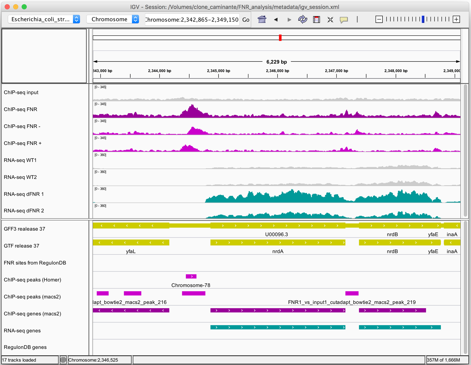
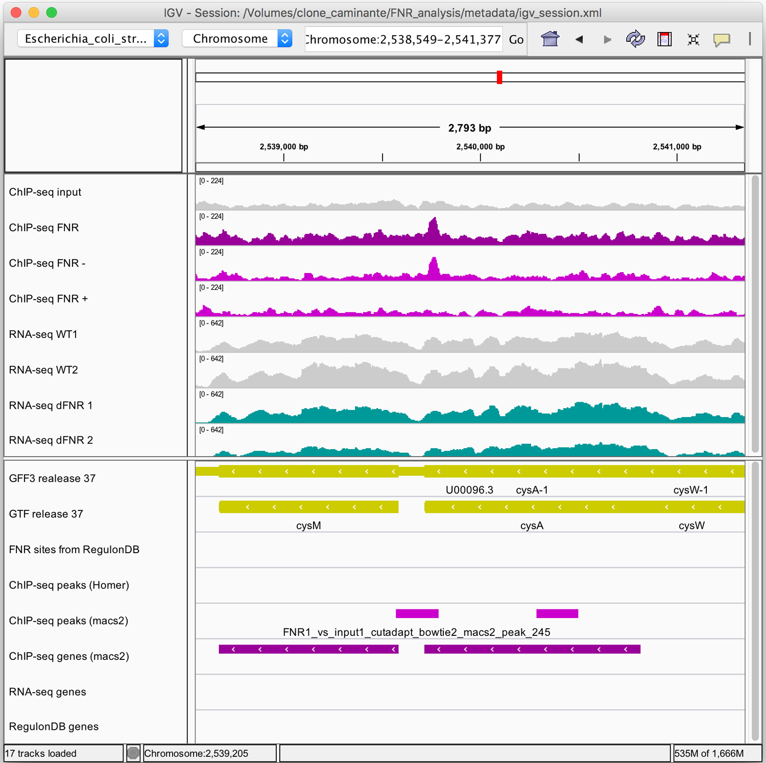
The figures were generated with the Integrative Genome Viewer (IGV). (a) High-confidence peak in the promoter region of the nrdAB operon. Note the characteristic shift between reads mapped on the + and - strand. (b) Example of peak that is likely to be a false positive. For both IGV maps (a, b): Top panel: coordinates of the displayed genomic region. Middle panel: read density profiles in the input (grey) and ChIP-seq sample (purple for strand-insensitive, pink for strand-sensitive profiles), and RNA-seq data (WT in grey, FNR mutants in turquoise). Lower panel: annotations tracks for genes (yellow), annotated FNR binding sites (none found in the displayed regions) and the binding peaks.

ChIP-seq (Basic Protocol 2)

Peak-calling

The peaks detected by Homer and Macs2 can be visualized in IGV as BED files. This file format contains essentially the coordinates of the regions with a high density of mapped reads, which are called peaks. While in bacteria it is expected for ChIP-seq peaks to fall into intergenic regions upstream of the regulated genes, it has been shown that a surprisingly high amount of binding could occur into coding or downstream regions (Galagan et al., 2012). This observation should be interpreted by taking into account the fact that bacteria have a very small amount of intergenic regions (10 to 15% of the genome).

Figure 10a shows a very clear peak around position 2,344,000, detected by both peak-callers, in the non-coding region upstream of the nrdA gene. By comparing the ChIP-seq read coverage on the forward and reverse strands (pink tracks in the middle panel), we see a shift between forward and reverse peaks. This typical pattern is consistent with the expectation for ChIP-seq experiments, since immunoprecipitated fragments are sequenced at their extremities, so that the reads are expected to be found either on the forward strand on the left of the binding site, or on the reverse strand on its right.

Alternative peak-calling tools can produce very different results on a same dataset. In the same region (Figure 10a), Macs2 detects another peak around position 2,347,000, associated to the nrdB gene, which pertains to the same operon as nrdA. It is not identified as a peak by Homer, and it is not associated to any known FNR TFBS from RegulonDB. However, RegulonDB indicates that nrdB is regulated by H-NS and Fis, nucleoid-associated proteins (NAPs) which are known to mask FNR binding sites under anaerobic conditions (Myers et al., 2013). Albeit barely detected by peak callers, this site is thus supported by some experimental evidence.

In contrast, Figure 10b shows a typical example of peak likely to be a false positive. Note that the read enrichment is restricted to the reverse strand, and falls within the coding region of a gene. Strand-specific display of read coverages thus enables to assess the reliability of peaks by inspecting their repartition around the putative binding sites.

The number of peaks and their width can vary a lot, hence the need to adapt the tools to a given study, and assess the relevance of the downstream results. With our working conditions, Homer returns 161 peaks of equal width (exactly 177 bp each), whereas macs2 returns 411 peaks ranging from 200 to 5893 bp (with and average of 475 bp), an obviously excessive size for transcription factor binding sites. The broadest peaks reported by macs2 correspond to wide regions covering several genes, which are entirely covered by reads in the ChIP-seq sample, and indeed enriched with respect to the genomic input, but which likely do not correspond to TF binding sites. For macs2, the number of peaks can be strongly modified by tuning the qvalue threshold and the minimal fold change. For example, the number of peaks drops from 547 with a qvalue threshold of 0.05 and a minimal fold-change of 2, to 159 with q-value threshold of 0.001 and a minimal fold-change of 5. The most lenient conditions give less relevant peaks, denoted by a drop of significance of the FNR motif. In summary, the choice of a peak-calling algorithm and the fine-tuning of its parameter crucially affect ChIP-seq results, and should be evaluated on a case-by-case basis.

Motif discovery in peak sequences

The top panel of Figure 11 shows the most significant motif returned by RSAT peak-motifs (Thomas-Chollier et al., 2012) in the sequences of Homer peaks. This motif was discovered by the tool dyad-analysis (van Helden et al., 2000), which detects over-represented pairs of spaced oligonucleotides. This motif discovery approach is particularly relevant for bacteria, where most transcription factors form homodimers that bind spaced motifs. The comparison of this discovered motif with all the TF binding motifs annotated in RegulonDB returns two matches, corresponding to FNR and CRP, respectively. The alignment highlights the strong similarity between the motifs recognized by FNR and CRP (they differ only by one nucleotide at position 7 of the motif alignment), which is consistent with the fact that these two factors are known to co-regulate a number of genes (Myers et al., 2013; Gama-Castro et al., 2016).

Figure 11.

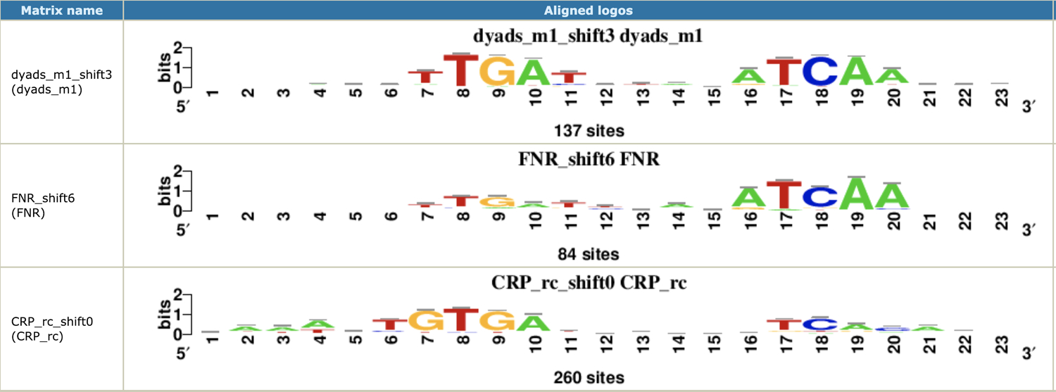
Most significant motif discovered by RSAT peak-motifs in the FNR peaks, aligned with matching motifs in RegulonDB.

RNA-seq (Basic Protocol 3)

Differentially expressed genes

The results of the RNA-seq analysis are summarized in an HTML report (RNA-seq/results/diffexpr/cutadapt_bwa_featureCounts_rna-seq_deg_report.html). which can be visualized using a web browser. It features information and statistics about the RNA-seq samples, read counts, and the differentially expressed genes, detected by using two different tools: DESeq2 (Love et al., 2014) and edgeR (Robinson et al., 2010). Figure 12 shows MA plots and volcano plots that are automatically produced by the workflow to provide a synthetic representation of the global results of the RNA-seq differential analysis. The MA plots (Figure 12a) indicate the relationship between the mean level of expression of each gene (abcsissa) and its differential expression, measured as the log-fold change between FNR mutant and wild type (ordinate). The genes declared differentially expressed between the two conditions (WT versus FNR) are highlighted as blue crosses. Genes over-expressed (respectively under-expressed) in the FNR mutants appear above (respectively below) the X-axis. The volcano plots (Figure 12b) provide a combined view of the expression changes (log fold change on the abscissa) and the statistical significance of these changes (ordinate). The significance is computed as the minus logarithm of the adjusted p-value reported by DESeq2 (left) and edgeR (right), respectively. High values are indicative of significant differences of expression between FNR mutant and WT strains. To select differentially expressed genes, SnakeChunks combines user-modifiable thresholds on the adjusted p-value (default: alpha = 0.05) and on the fold change (default: at least 2-fold over- or under-expression).

Figure 12. Global views of the results for the detection of differentially expressed genes between FNR mutant versus wild-type.

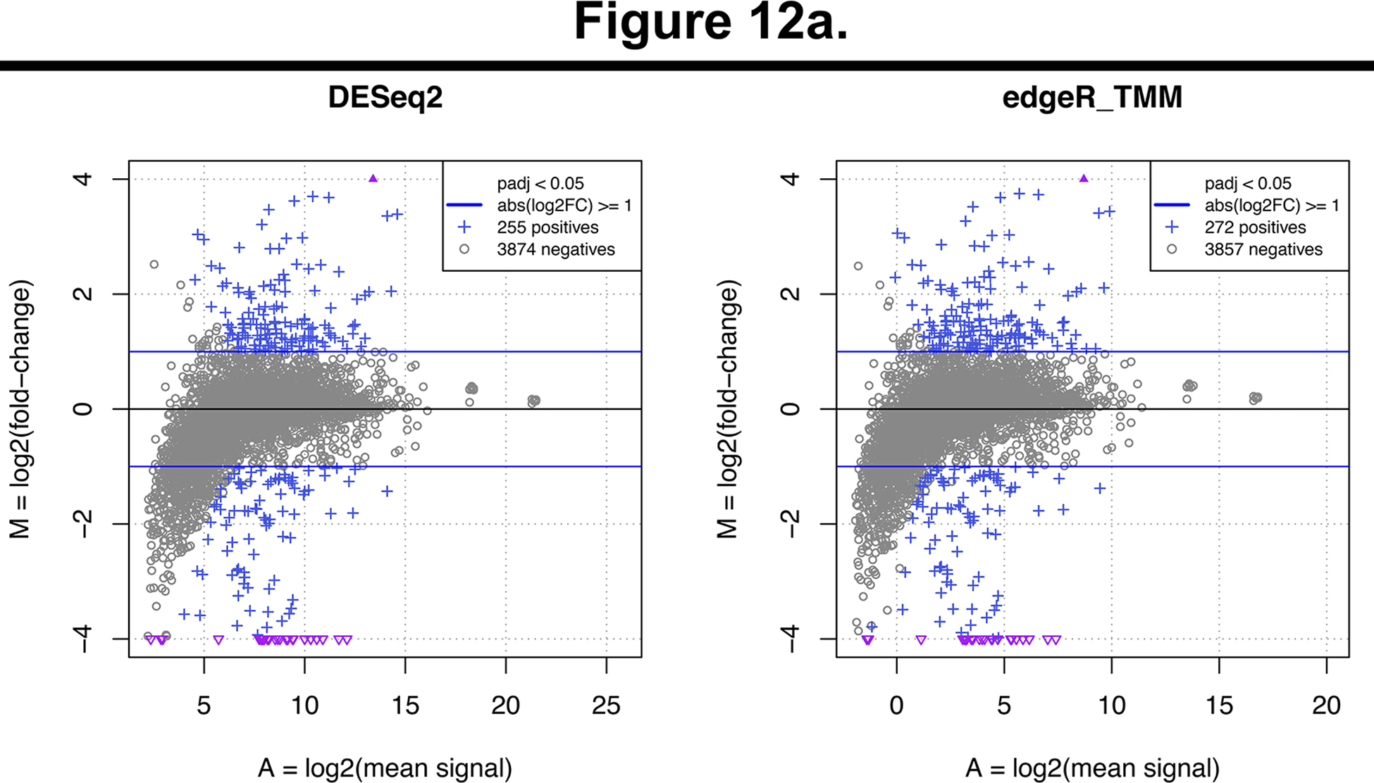
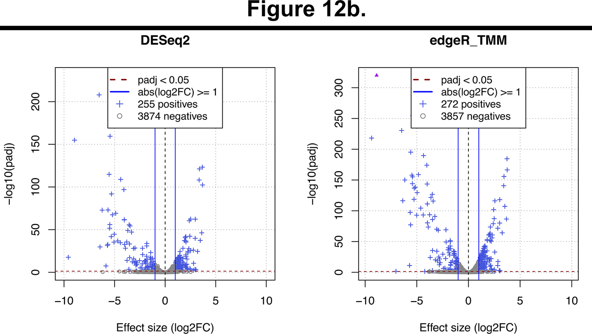
These plots are generated as part of the differential analysis step, using an R script. Left and right panels respectively show the results of DESeq2 and edgeR. (a) MA plots. The abscissa indicates the mean level of expression (average of the log-transformed counts), the ordinate shows the log-fold change between FNR mutant and wild-type strain, which indicates the level of over- (positive values) or under-expression (negative values). Differentially Expressed Genes (DEG), i.e. those passing both thresholds on effect size and significance, are highlighted in blue. Triangles indicate genes whose log2 fold-change exceed the plot limits. (b) Volcano plots. The abscissa represents the log-fold change, which indicates the size of the effect, and its sign (“-”: down-regulation; “+”: up-regulation). The ordinate shows the significance of the differential expression (minus log of the adjusted p-value).

In total, these thresholds lead to retain 278 differentially expressed genes (DEG), which are declared positive by either DESeq2 (255 genes) or edgeR (272 genes). This number is consistent with the fact that FNR acts as global regulator in E.coli. Note that we chose to keep the union of both lists in order to favour sensitivity, but this can be parametrized in the configuration file, by specifying that DEG detection relies on edgeR, DESeq2, their intersection or their union.

Integration (Basic Protocol 4)

The Venn diagram generated by the workflow (Figure 13, file integration/ChIP-RNA-regulons_venn.png) shows the number of E.coli genes associated to FNR peaks in the ChIP-seq experiment (pink), reported as differentially expressed in the RNA-seq analysis (green), or annotated as FNR targets in RegulonDB (violet), as well as the intersections between these gene sets. Depending on the peak-calling algorithm, the number of genes found at the intersection between the three gene lists (ChIP-seq, RNA-seq and RegulonDB) is quite small (38 for macs2 peaks and 28 for Homer peaks) relative to the respective size of the compared gene sets. It is interesting to get an interpretive guideline for the pairwise intersections or set memberships. The genes reported by both ChIP-seq (FNR binding) and RNA-seq (FNR transcriptional response) but not annotated in RegulonDB are likely to be direct FNR target genes, and might be considered to be added to RegulonDB, in an annotation track based on combined evidence from complementary high-throughput experiments. This would give 29 genes with macs2 peaks, and 25 with Homer peaks. It would be interesting to furthermore scan their promoter sequences in order to search instances of the FNR binding motif in order to predict binding site locations, and consolidate the results. The 160 genes (rep 167) detected by macs2 (resp Homer) as differentially expressed without any associated peak nor annotated FNR site include genes located inside the target operons of FNR. Indeed, in bacteria, polycistronic transcripts are regulated by cis-acting elements located in the promoter of the operon-leader gene. Consistently, 38 of these genes (~23%) have a very short upstream non-coding region (<55bp) typical of intra-operon genes, whereas almost all the genes of the triple intersection (28 among 29) have larger upstream sequences typical of operon-leader genes. The remaining 77% of differentially expressed genes without associated ChIP-seq peak are likely to be indirect FNR targets, whose transcription might be affected via intermediate transcription factors themselves regulated by FNR. The genes associated with ChIP-seq peaks without transcriptional response (334 for macs2, 119 for Homer) likely result from different effects: non-functional binding of the FNR factor in the experimental conditions of the study (missing co-activator, co-binding of a repressor), binding between two divergently transcribed transcription units, but regulating only one of them, or false positives of the peak calling (e.g. regions with a high density of reads on one strand only, as discussed above).

Figure 13. Integration of ChIP-seq, RNA-seq results and RegulonDB annotations.

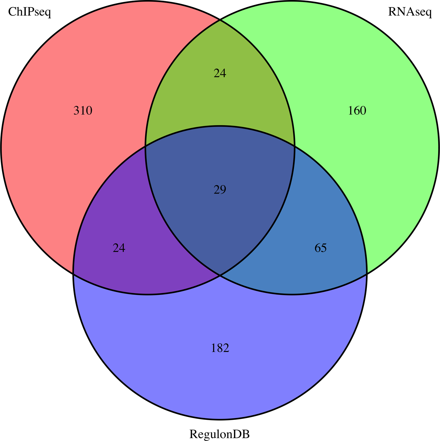
Venn diagrams showing the intersection of the genes linked to ChIP-seq peaks (pink), those declared differentially expressed by RNA-seq experiment (green) and those annotated as FNR target genes in RegulonDB (violet). These diagrams are automatically generated by the integration workflow, using the R library VennDiagram. (a) Results with the 411 ChIP-seq peaks reported by macs2 with qvalue < 0.01 and fold-change between 2 and 50. (b) Results with the 166 ChIP-seq peaks reported by Homer.

Figure 14 highlights some illustrative examples of differentially expressed genes detected by DESeq2 or edgeR. For the cydABX operon (Figure 14a), the FNR mutant (jade tracks on the genome coverage profiles) has an increased level of expression than the wild-type (gray tracks). Consistently, this operon has been demonstrated to be repressed by FNR (Salmon et al., 2003), and has two annotated FNR binding sites in RegulonDB, which overlap a strong peak detected by both Homer and Macs2 in the ChIP-seq results.

Figure 14. IGV snapshots of RNA-seq results for three illustrative operons.

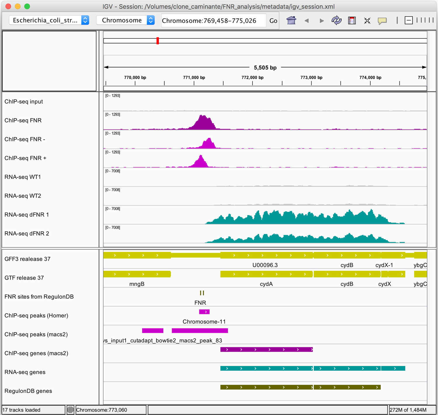
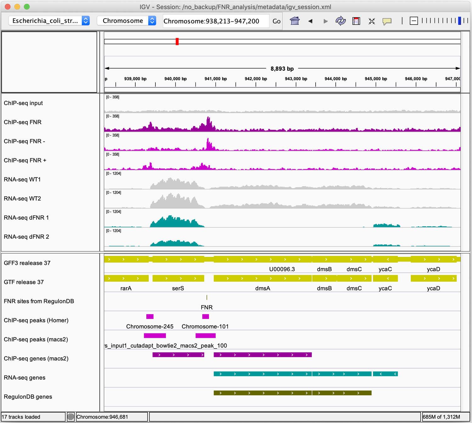
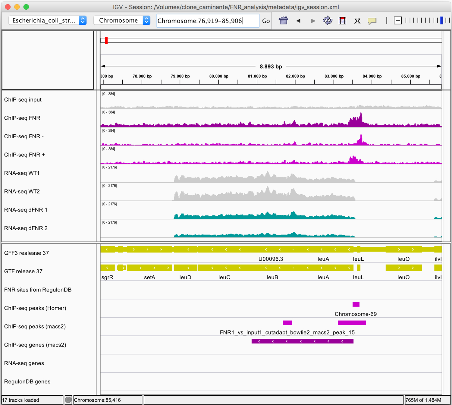
Middle panel: genome coverage profiles for the two replicas of the wild-type (grey) and FNR mutant (jade). Lower panel: genome annotations for the genes (yellow), FNR binding sites from RegulonDB (grey), differentially expressed genes (jade) and FNR target genes annotated in RegulonDB (dark olive). Views of selected regions encompassing (a) the cydABX operon (b) the dmsABC operon (c) the leuLABCD operon.

The dmsABC operon also exemplifies the genes found at the triple intersection: it has been shown to be regulated by FNR (Melville and Gunsalus, 1996), and, consistently, it has one TFBS listed in RegulonDB, and is reported by both the ChIP-seq and RNA-seq experiments (Figure 14b).

A more subtle example is the leuLABCD operon (Figure 14c): RNA-seq coverage profiles also reveal a reduced expression, although the differential expression analysis didn’t report any significant gene, due to the stringent thresholds applied on both adjusted p-value (< 0.05) and fold change (>2). This operon encodes the enzymes responsible for the biosynthesis of leucine from valine. It has no binding sites annotated in RegulonDB for the FNR transcription factor, and based on the RNA-seq results only, several possibilities could be invoked to explain this inconsistency: the leu operon might be (i) indirectly regulated by FNR via another transcription factor; (ii) under a direct target of FNR whose binding sites have not been characterized yet; (iii) or it could be a false-positive. This situation can be clarified by analysing the ChIP-seq profiles, since we can observe a clear peak upstream of the operon, detected by both macs2 and Homer (Figure 14c), enforcing the evidences for a direct regulation of the leu operon by FNR.

In summary, a detailed analysis and human-based interpretation of combined RNA-seq and ChIP-seq data is worth to go beyond the gene lists returned by the automatic comparison of target genes predicted by ChIP-seq and RNA-seq experiments.

COMMENTARY

Background Information

Next Generation Sequencing (NGS) technologies (Schuster, 2007) emerged in 2007 with the development of several approaches for massively parallel sequencing of short DNA sequences (a few tens of base pairs per sequence). This unprecedented gain in sequencing speed was mobilised for a wide variety of applications: genome sequencing, transcriptome (RNA-seq), genome-wide binding location analysis (ChIP-seq), chromatin conformation (Hi-C), metagenomics, and many others. Research projects based on NGS typically lead to the situation where the biologist performs experiments, sends the samples to a sequencing center, and receives a link to download several Gigabases of raw sequences called “short reads”. Since 2007, a wide variety of software tools was developed to handle NGS data and extract relevant information (Pepke et al., 2009).

Proper use of such software requires a good understanding of their parameters, strengths and weaknesses. Beyond the choice and parametrization of each particular tool, it became crucial to formalise their wiring by implementing workflows that ensure traceability and reproducibility of all the steps used to produce the results from the raw data. Many alternative software systems can be used to manage the development and execution of analysis workflows. Among them, Galaxy (Goecks, 2010) became highly popular because it offers an immediate access through a graphical interface to biologists with no experience in the Unix terminal. Snakemake (Köster and Rahmann, 2012) offers a complementary solution to achieve the same goals — developing, managing and running NGS workflows — in the Unix command line environment. Snakemake is currently being adopted by a growing number of bioinformaticians as well as experimental biologists willing to get one step further in the analysis of their own data. The goal of SnakeChunks is to facilitate the conception and use of NGS workflows by encapsulating Snakemake commands in a library of modular rules (one per tool) that can be combined in various ways to build and customize workflows (Figure 2).

Critical Parameters

Control samples

When analysing binding signal (ChIP-seq) or transcription signal (RNA-seq), it is crucial to generate appropriate control experiments, in order to measure differences in signal against a proper background signal, and thus avoid the detection of false positives. This is especially important when analysing ChIP-seq data, since false peaks can arise from biases in the experiments: non-homogeneous sonication of DNA due non-homogeneous aperture of the chromatin, GC biases arising during PCR amplification of the fragments, low-complexity regions of the genome… Different types of controls can be used to estimate the background probabilities of read mapping in the different regions of the genome: (1) sequencing genomic DNA without immunoprecipitation; (2) “mock IP” consists in performing the immunoprecipitation with a non-specific antibody; (3) another possibility is to artificially knock-out the expression of the TF of interest. Irrespective of the method used, the control sequences are generally denoted as “input” for the peak-calling programs. In the study by Myers and colleagues, genomic DNA was used as input. In the case of RNA-seq, knocked-out TFs or over-expressed TFs can be compared against WT samples. In this study, samples with an inactivated FNR protein were compared against WT strains.

Number of replicates

When performing biological experiments, it is crucial to account for the unavoidable variability intrinsic to living organisms. RNA-seq experiments are no exception, and it has been demonstrated that the higher the number of replicates, the more sensitive the detection of differentially expressed genes (Schurch et al., 2016). Designing experiments with a high number of replicates enables the analysis to distinguish subtle but relevant changes in expression from spurious fluctuations due to biological variability.

Choice of a read mapper

Read mapping is generally the most consuming task of RNA-seq and ChIP-seq data analysis. For the FNR study case developed in this article, the complete ChIP-seq workflow runs in a few minutes, whereas the RNA-seq workflows takes several hours. The modularity of the SnakeChunks library enabled us to run the same workflow with three alternative read-mapping tools: BWA (Li et al., 2009), bowtie2 (Langmead et al, 2012) and subread-align (Liao et al., 2013). For this particular dataset, BWA runs approximately 3 times faster than the two other algorithms, while giving very similar mapping rates. However, we experienced opposite rankings of performances with other datasets and reference genomes. The choice and parametrization of a read mapper should thus be considered as critical step, which has to be tuned in a case-specific way to optimise a workflow.

Troubleshooting

The Snakemake workflow management system is equipped with its own mechanisms for detecting, reporting and fixing problems. Trouble is reported with red messages displayed on the terminal indicating the kind of problems and — when possible — the suggested ways to fix them.

Advanced Parameters

A proper parametrization of the workflow is the key to optimise both computing efficiency and biological relevance of the results.

Parameters can be changed either by modifying the YAML-formatted configuration file in the metadata (see section Support Protocol 1: Customization of the Parameters), or with the option --config in the Snakemake command line (see example in section Basic Protocol 1, step 3).

With the popularisation of RNA-seq for transcriptome studies, the number of samples per research project has been expanding in recent publications. Crucial parameter will be the capability to keep with the increased needs of storage, and to parallelize computation for large studies. The FNR study case treated for this protocol was intently selected for its small number of replicates per condition, but for wider-scale studies the number of simultaneous jobs handled by snakemake should be adapted to the number of CPUs of the computing system (option -j option).

We also make a frequent use of the snakemake option -n, which prints out all the commands required to complete a workflow, without actually executing them (“dry run”). This gives the user the possibility to check that a command is properly parametrized before running, which can be valuable when handling hour-lasting tasks on multiple samples.

Suggestions for Further Analysis

The main goal of the SnakeChunks library is to ensure the reproducibility of the analyses. This is why we recommend keeping a copy of the library with each dataset analysed in order to ensure consistency between the results and the precise version of the library used to generate them. This is particularly crucial in case of publication, so readers can actually reproduce the analyses performed.

The use of conda also enables the user to keep control over the software environment, and is in accordance with the FAIR principles (Wilkinson et al., 2016).

A natural extension of this work will be to take advantage of SnakeChunks’ flexibility in order to assess the impact of tool and parametric choices on the biological relevance of the results, and to optimise workflows by evaluating the correspondence between the lists of genes returned by combining ChIP-seq and RNA-seq results and those already annotated in RegulonDB for well-characterised transcription factors.

Significance Statement.

Next-Generation Sequencing (NGS) is revolutionizing all domains of life sciences, from health to agriculture and environment. A crucial issue for big data science is to ensure the reproducibility of the results. This applies to biological experiments as well as bioinformatics processing, since the conclusions of a study can change drastically depending on the tools used, their parameterization, the full availability of the data and the proper organisation of the data files. To manage massive amounts of data, NGS-based research relies on complex successions of computing tasks. Here, we present a software library enabling to design and customize workflows to perform reproducible ChIP-seq and RNA-seq analyses, illustrated by a study case in the model organism Escherichia coli.

INTERNET RESOURCES

1. SnakeMake: http://snakemake.readthedocs.io

2. SnakeChunks github repository: https://github.com/SnakeChunks/SnakeChunks

3. SnakeChunks documentation & tutorials: http://snakechunks.readthedocs.io

4. FastQC: http://www.bioinformatics.babraham.ac.uk/projects/fastqc/

5. UCSC file format description: https://genome.ucsc.edu/FAQ/FAQformat.html

LITERATURE CITED

- Andrews S (2010). FastQC: a quality control tool for high throughput sequence data. Available online at: http://www.bioinformatics.babraham.ac.uk/projects/fastqc [Google Scholar]
- Angelini C, & Costa V (2014). Understanding gene regulatory mechanisms by integrating ChIP-seq and RNA-seq data: statistical solutions to biological problems. Frontiers in Cell and Developmental Biology. 10.3389/fcell.2014.00051 [DOI] [PMC free article] [PubMed] [Google Scholar]
- Aquino P, Honda B, Jaini S, Lyubetskaya A, Hosur K, Chiu JG, Ekladious I, Hu D, Jin L, Sayeg MK, Stettner AI, Wang J, Wong BG, Wong WS, Alexander SL, Ba C, Bensussen SI, Bernstein DB, Braff D, Cha S, Cheng DI, Cho JH, Chou K, Chuang J, Gastler DE, Grasso DJ, Greifenberger JS, Guo C, Hawes AK, Israni DV, Jain SR, Kim J, Lei J, Li H, Li D, Li Q, Mancuso CP, Mao N, Masud SF, Meisel CL, Mi J, Nykyforchyn CS, Park M, Peterson HM, Ramirez AK, Reynolds DS, Rim NG, Saffie JC, Su H, Su WR, Su Y, Sun M, Thommes MM, Tu T, Varongchayakul N, Wagner TE, Weinberg BH, Yang R, Yaroslavsky A, Yoon C, Zhao Y, Zollinger AJ, Stringer AM, Foster JW, Wade J, Raman S, Broude N, Wong WW, Galagan JE (2017). Coordinated regulation of acid resistance in Escherichia coli. BMC Systems Biology. 10.1186/s12918-016-0376-y [DOI] [PMC free article] [PubMed] [Google Scholar]
- Bailey T, Krajewski P, Ladunga I, Lefebvre C, Li Q, Liu T, Madrigal P, Taslim C, Zhang J (2013). Practical Guidelines for the Comprehensive Analysis of ChIP-seq Data. PLoS Computational Biology. 10.1371/journal.pcbi.1003326 [DOI] [PMC free article] [PubMed] [Google Scholar]
- Birney E (2012). The making of ENCODE: Lessons for big-data projects. Nature. 10.1038/489049a [DOI] [PubMed] [Google Scholar]
- Blattner FR, Plunkett G, Bloch CA, Perna NT, Burland V, Riley M, Collado-Vides J, Glasner JD, Rode CK, Mayhew GF, Gregor J, Davis NW, Kirkpatrick HA, Goeden MA, Rose DJ, Mau B, Shao Y (1997). The complete genome sequence of Escherichia coli K-12. Science (New York, N.Y.), 277(5331), 1453–1462. [DOI] [PubMed] [Google Scholar]
- Cadby IT, Faulkner M, Cheneby J, Long J, van Helden J, Dolla A, & Cole JA (2017). Coordinated response of the Desulfovibrio desulfuricans 27774 transcriptome to nitrate, nitrite and nitric oxide. Scientific Reports, 7(1), 16228 10.1038/s41598-017-16403-4 [DOI] [PMC free article] [PubMed] [Google Scholar]
- Castro-Mondragon JA, Rioualen C, Contreras-Moreira B, & van Helden J (2016). RSAT::Plants: Motif discovery in ChIP-seq peaks of plant genomes (Vol. 1482). [DOI] [PubMed] [Google Scholar]
- Desvillechabrol D, Legendre R, Rioualen C, Bouchier C, van Helden J, Kennedy S, & Cokelaer T (2018). Sequanix: a dynamic graphical interface for Snakemake workflows. Bioinformatics, 34(11), 1934–1936. 10.1093/bioinformatics/bty034 [DOI] [PMC free article] [PubMed] [Google Scholar]
- Diaz A, Park K, Lim DA, & Song JS (2012). Normalization, bias correction, and peak calling for ChIP-seq. Statistical Applications in Genetics and Molecular Biology. 10.1515/1544-6115.1750 [DOI] [PMC free article] [PubMed] [Google Scholar]
- Dongjun Chung A, Fen Kuan P, Welch R, & Keles Maintainer Dongjun Chung S (2017). Package “mosaics” Title MOSAiCS (MOdel-based one and two Sample Analysis and Inference for ChIP-Seq).
- Feng J, Liu T, & Zhang Y (2011). Using MACS to identify peaks from ChiP-seq data. Current Protocols in Bioinformatics. 10.1002/0471250953.bi0214s34 [DOI] [PMC free article] [PubMed] [Google Scholar]
- Galagan J, Lyubetskaya A, & Gomes A (2012). ChIP-Seq and the Complexity of Bacterial Transcriptional Regulation In Systems Biology (pp. 43–68). Springer, Berlin, Heidelberg: Retrieved from https://link.springer.com/chapter/10.1007/82_2012_257 [DOI] [PubMed] [Google Scholar]
- Galagan JE, Minch K, Peterson M, Lyubetskaya A, Azizi E, Sweet L, Gomes A, Rustad T, Dolganov G, Glotova I, Abeel T, Mahwinney C, Kennedy AD, Allard R, Brabant W, Krueger A, Jaini S, Honda B, Yu WH, Hickey MJ, Zucker J, Garay C, Weiner B, Sisk P, Stolte C, Winkler JK, Van de Peer Y, Iazzetti P, Camacho D, Dreyfuss J, Liu Y, Dorhoi A, Mollenkopf HJ, Drogaris P, Lamontagne J, Zhou Y, Piquenot J, Park ST, Raman S, Kaufmann SH, Mohney RP, Chelsky D, Moody DB, Sherman DR, Schoolnik GK (2013). The Mycobacterium tuberculosis regulatory network and hypoxia. Nature. 10.1038/nature12337 [DOI] [PMC free article] [PubMed] [Google Scholar]
- Gama-Castro S, Salgado H, Santos-Zavaleta A, Ledezma-Tejeida D, Muñiz-Rascado L, García-Sotelo JS, Alquicira-Hernández K, Martínez-Flores I, Pannier L, Castro-Mondragón JA, Medina-Rivera A, Solano-Lira H, Bonavides-Martínez C, Pérez-Rueda E, Alquicira-Hernández S, Porrón-Sotelo L, López-Fuentes A, Hernández-Koutoucheva A, Del Moral-Chávez V, Rinaldi F, Collado-Vides J (2016). RegulonDB version 9.0: high-level integration of gene regulation, coexpression, motif clustering and beyond. Nucleic Acids Research, 44(D1), D133–143. 10.1093/nar/gkv1156 [DOI] [PMC free article] [PubMed] [Google Scholar]
- Goecks J, Nekrutenko A, Taylor J; Galaxy Team. Galaxy: a comprehensive approach for supporting accessible, reproducible, and transparent computational research in the life sciences. Genome Biol. 2010;11(8):R86. doi: 10.1186/gb-2010-11-8-r86. [DOI] [PMC free article] [PubMed] [Google Scholar]
- Grainger DC, Aiba H, Hurd D, Browning DF, & Busby SJW (2007). Transcription factor distribution in Escherichia coli: Studies with FNR protein. Nucleic Acids Research. 10.1093/nar/gkl1023 [DOI] [PMC free article] [PubMed] [Google Scholar]
- Heinz S, Benner C, Spann N, Bertolino E, Lin YC, Laslo P, Cheng JX, Murre C, Singh H, Glass CK (2010). Simple Combinations of Lineage-Determining Transcription Factors Prime cis-Regulatory Elements Required for Macrophage and B Cell Identities. Molecular Cell, 38(4), 576–589. 10.1016/j.molcel.2010.05.004 [DOI] [PMC free article] [PubMed] [Google Scholar]
- Jacob F, & Monod J (1961). Genetic regulatory mechanisms in the synthesis of proteins. Journal of Molecular Biology, 3, 318–356. [DOI] [PubMed] [Google Scholar]
- Johnson DS, Mortazavi A, Myers RM, & Wold B (2007). Genome-wide mapping of in vivo protein-DNA interactions. Science (New York, N.Y.), 316(5830), 1497–1502. 10.1126/science.1141319 [DOI] [PubMed] [Google Scholar]
- Köster J, & Rahmann S (2012). Snakemake-a scalable bioinformatics workflow engine. Bioinformatics. 10.1093/bioinformatics/bts480 [DOI] [PubMed] [Google Scholar]
- Landt SG, Marinov GK, Kundaje A, Kheradpour P, Pauli F, Batzoglou S, Bernstein BE, Bickel P, Brown JB, Cayting P, Chen Y, DeSalvo G, Epstein C, Fisher-Aylor KI, Euskirchen G, Gerstein M, Gertz J, Hartemink AJ, Hoffman MM, Iyer VR, Jung YL, Karmakar S, Kellis M, Kharchenko PV, Li Q, Liu T, Liu XS, Ma L, Milosavljevic A, Myers RM, Park PJ, Pazin MJ, Perry MD, Raha D, Reddy TE, Rozowsky J, Shoresh N, Sidow A, Slattery M, Stamatoyannopoulos JA, Tolstorukov MY, White KP, Xi S, Farnham PJ, Lieb JD, Wold BJ, Snyder M (2012). ChIP-seq guidelines and practices of the ENCODE and modENCODE consortia. Genome Research. 10.1101/gr.136184.111 [DOI] [PMC free article] [PubMed] [Google Scholar]
- Langmead B, Salzberg SL. (2012). Fast gapped-read alignment with Bowtie 2. Nat Methods. 2012 Mar 4;9(4):357–9. doi: 10.1038/nmeth.1923. [DOI] [PMC free article] [PubMed] [Google Scholar]
- Lazazzera BA, Bates DM, & Kiley PJ (1993). The activity of the Escherichia coli transcription factor FNR is regulated by a change in oligomeric state. Genes & Development, 7(10), 1993–2005. 10.1101/gad.7.10.1993 [DOI] [PubMed] [Google Scholar]
- Li H and Durbin R (2009) Fast and accurate short read alignment with Burrows-Wheeler Transform. Bioinformatics, 25:1754–60. [DOI] [PMC free article] [PubMed] [Google Scholar]
- Liang K, & Uz Kele U (2012). Normalization of ChIP-seq data with control, 13 Retrieved from http://www.biomedcentral.com/1471-2105/13/199 [DOI] [PMC free article] [PubMed] [Google Scholar]
- Liao Y, Smyth GK and Shi W. (2013). The Subread aligner: fast, accurate and scalable read mapping by seed-and-vote. Nucleic Acids Research, 41(10):e108. [DOI] [PMC free article] [PubMed] [Google Scholar]
- Liao Y, Smyth GK and Shi W. (2013). featureCounts: an efficient general-purpose program for assigning sequence reads to genomic features. Bioinformatics, 30(7):923–30. [DOI] [PubMed] [Google Scholar]
- Love MI, Huber W and Anders S (2014). Moderated estimation of fold change and dispersion for RNA-seq data with DESeq2. Genome Biology, 15, pp. 550. doi: 10.1186/s13059-014-0550-8. [DOI] [PMC free article] [PubMed] [Google Scholar]
- Lun DS, Sherrid A, Weiner B, Sherman DR, & Galagan JE (2009). A blind deconvolution approach to high-resolution mapping of transcription factor binding sites from ChIP-seq data. Genome Biology. 10.1186/gb-2009-10-12-r142 [DOI] [PMC free article] [PubMed] [Google Scholar]
- Martin M Cutadapt removes adapter sequences from high-throughput sequencing reads. EMBnet.journal, [S.l.], v. 17, n. 1, p. pp. 10–12, May 2011. ISSN 2226–6089. Available at: http://journal.embnet.org/index.php/embnetjournal/article/view/200. [Google Scholar]
- Melville SB, & Gunsalus RP (1996). Isolation of an oxygen-sensitive FNR protein of Escherichia coli: interaction at activator and repressor sites of FNR-controlled genes. Proceedings of the National Academy of Sciences of the United States of America, 93(3), 1226–1231. [DOI] [PMC free article] [PubMed] [Google Scholar]
- Merhej J, Frigo A, Le Crom S, Camadro JM, Devaux F, & Lelandais G (2014). bPeaks: A bioinformatics tool to detect transcription factor binding sites from ChIP-seq data in yeasts and other organisms with small genomes. Yeast. 10.1002/yea.3031 [DOI] [PubMed] [Google Scholar]
- Myers KS, Park DM, Beauchene NA, & Kiley PJ (2015). Defining bacterial regulons using ChIP-seq. Methods. 10.1016/j.ymeth.2015.05.022 [DOI] [PMC free article] [PubMed] [Google Scholar]
- Myers KS, Yan H, Ong IM, Chung D, Liang K, Tran F, Keleş S, Landick R, Kiley PJ (2013). Genome-scale Analysis of Escherichia coli FNR Reveals Complex Features of Transcription Factor Binding. PLoS Genetics, 9(6). 10.1371/journal.pgen.1003565 [DOI] [PMC free article] [PubMed] [Google Scholar]
- Nekrutenko A, & Taylor J (2012). Next-generation sequencing data interpretation: enhancing reproducibility and accessibility. Nature Reviews Genetics. 10.1038/nrg3305 [DOI] [PubMed] [Google Scholar]
- Ngoune JMT, Njiokou F, Loriod B, Kame-Ngasse G, Fernandez-Nunez N, Rioualen C, van Helden J, Geiger A (2017). Transcriptional profiling of midguts prepared from Trypanosoma/T. Congolense-positive Glossina palpalis palpalis collected from two distinct cameroonian foci: Coordinated signatures of the midguts’ remodeling as T. Congolense-supportive niches. Frontiers in Immunology, 8(JUL). 10.3389/fimmu.2017.00876 [DOI] [PMC free article] [PubMed] [Google Scholar]
- Nguyen NTT, Contreras-Moreira B, Castro-Mondragon JA, Santana-Garcia W, Ossio R, Robles-Espinoza CD, Bahin M, Collombet S, Vincens P, Thieffry D, van Helden J, Medina-Rivera A, Thomas-Chollier M (2018). RSAT 2018: regulatory sequence analysis tools 20th anniversary. Nucleic Acids Research, 46(W1), W209–W214. 10.1093/nar/gky317 [DOI] [PMC free article] [PubMed] [Google Scholar]
- Pepke S, Wold B, & Mortazavi A (2009). Computation for ChIP-seq and RNA-seq studies. Nature Methods. 10.1038/nmeth.1371 [DOI] [PMC free article] [PubMed] [Google Scholar]
- Pérez-Rueda E, & Collado-Vides J (2000). The repertoire of DNA-binding transcriptional regulators in Escherichia coli K-12. Nucleic Acids Research, 28(8), 1838–1847. [DOI] [PMC free article] [PubMed] [Google Scholar]
- Rioualen C, Charbonnier-Khamvongsa L, van Helden J (2017). SnakeChunks: modular blocks to build Snakemake workflows for reproducible NGS analyses. bioRxiv 165191; doi: 10.1101/165191 [DOI] [Google Scholar]
- Robertson G, Hirst M, Bainbridge M, Bilenky M, Zhao Y, Zeng T, Euskirchen G, Bernier B, Varhol R, Delaney A, Thiessen N, Griffith OL, He A, Marra M, Snyder M, Jones S (2007). Genome-wide profiles of STAT1 DNA association using chromatin immunoprecipitation and massively parallel sequencing. Nature Methods, 4(8), 651–657. 10.1038/nmeth1068 [DOI] [PubMed] [Google Scholar]
- Robinson JT, Thorvaldsdóttir H, Winckler W, Guttman M, Lander ES, Getz G, & Mesirov JP (2011). Integrative Genomics Viewer. Nature Biotechnology, 29(1), 24–26. 10.1038/nbt.1754 [DOI] [PMC free article] [PubMed] [Google Scholar]
- Robinson MD, McCarthy DJ, Smyth GK (2010). edgeR: a Bioconductor package for differential expression analysis of digital gene expression data. Bioinformatics, 26(1), 139–140. [DOI] [PMC free article] [PubMed] [Google Scholar]
- Salmon K, Hung S, Mekjian K, Baldi P, Hatfield GW, & Gunsalus RP (2003). Global Gene Expression Profiling in Escherichia coli K12 the effect of oxygen availability and FNR. Journal of Biological Chemistry, 278(32), 29837–29855. 10.1074/jbc.M213060200 [DOI] [PubMed] [Google Scholar]
- Schuster SC. (2007). Next-generation sequencing transforms today’s biology. Nat Methods. 2008 Jan;5(1):16–8. doi: 10.1038/nmeth1156. [DOI] [PubMed] [Google Scholar]
- Schurch NJ, Schofield P, Gierliński M, Cole C, Sherstnev A, Singh V, Wrobel N, Gharbi K, Simpson GG, Owen-Hughes T, Blaxter M, Barton GJ (2016). How many biological replicates are needed in an RNA-seq experiment and which differential expression tool should you use? RNA. 10.1261/rna.053959.115 [DOI] [PMC free article] [PubMed] [Google Scholar]
- Standards, Guidelines and Best Practices for RNA-Seq: 2010/2011. (2011).
- Stodden V, McNutt M, Bailey DH, Deelman E, Gil Y, Hanson B, Heroux MA, Ioannidis JP, Taufer M (2016). Enhancing reproducibility for computational methods. Science, 354(6317), 1240–1241. 10.1126/science.aah6168 [DOI] [PubMed] [Google Scholar]
- Thomas-Chollier M, Herrmann C, Defrance M, Sand O, Thieffry D, & Van Helden J (2012). RSAT peak-motifs: Motif analysis in full-size ChIP-seq datasets. Nucleic Acids Research. 10.1093/nar/gkr1104 [DOI] [PMC free article] [PubMed] [Google Scholar]
- Thorvaldsdóttir H, Robinson JT, & Mesirov JP (2013). Integrative Genomics Viewer (IGV): high-performance genomics data visualization and exploration. Briefings in Bioinformatics, 14(2), 178–192. 10.1093/bib/bbs017 [DOI] [PMC free article] [PubMed] [Google Scholar]
- van Helden, Ríos AF, Collado-Vides J (2000) “Discovering regulatory elements in non-coding sequences by analysis of spaced dyads” Nucleic Acids Res. 28(8): 1808–1818 [DOI] [PMC free article] [PubMed] [Google Scholar]
- Wilbanks EG, & Facciotti MT (2010). Evaluation of algorithm performance in ChIP-seq peak detection. PLoS ONE. 10.1371/journal.pone.0011471 [DOI] [PMC free article] [PubMed] [Google Scholar]
- Wilkinson MD, Dumontier M, Aalbersberg Ij. J., Appleton G, Axton M, Baak A, Blomberg N, Boiten JW, da Silva Santos LB, Bourne PE, Bouwman J, Brookes AJ, Clark T, Crosas M, Dillo I, Dumon O, Edmunds S, Evelo CT, Finkers R, Gonzalez-Beltran A, Gray AJ, Groth P, Goble C, Grethe JS, Heringa J, ‘t Hoen PA, Hooft R, Kuhn T, Kok R, Kok J, Lusher SJ, Martone ME, Mons A, Packer AL, Persson B, Rocca-Serra P, Roos M, van Schaik R, Sansone SA, Schultes E, Sengstag T, Slater T, Strawn G, Swertz MA, Thompson M, van der Lei J, van Mulligen E, Velterop J, Waagmeester A, Wittenburg P, Wolstencroft K, Zhao J, Mons B (2016, March 15). The FAIR Guiding Principles for scientific data management and stewardship [Comments and Opinion]. Retrieved December 1, 2017, from https://www.nature.com/articles/sdata20161 [DOI] [PMC free article] [PubMed]
Associated Data
This section collects any data citations, data availability statements, or supplementary materials included in this article.