Correction of respiratory artifacts in MRI head motion estimates

Abstract

Head motion represents one of the greatest technical obstacles in magnetic resonance imaging (MRI) of the human brain. Accurate detection of artifacts induced by head motion requires precise estimation of movement. However, head motion estimates may be corrupted by artifacts due to magnetic main field fluctuations generated by body motion. In the current report, we examine head motion estimation in multiband resting state functional connectivity MRI (rs-fcMRI) data from the Adolescent Brain and Cognitive Development (ABCD) Study and comparison ‘single-shot’ datasets. We show that respirations contaminate movement estimates in functional MRI and that respiration generates apparent head motion not associated with functional MRI quality reductions. We have developed a novel approach using a band-stop filter that accurately removes these respiratory effects from motion estimates. Subsequently, we demonstrate that utilizing a band-stop filter improves post-processing fMRI data quality. Lastly, we demonstrate the real-time implementation of motion estimate filtering in our FIRMM (Framewise Integrated Real-Time MRI Monitoring) software package.

Introduction

Head motion represents one of the greatest technical obstacles in magnetic resonance imaging (MRI). In both task-driven fMRI (t-fMRI) and resting state functional connectivity MRI (rs-fcMRI), even sub-millimeter head movements (i.e., micro-movements) introduce artifact, thereby corrupting the data in both typical and atypical populations (Fair et al., 2013; Power et al., 2012; Satterthwaite et al., 2012; Van Dijk et al., 2012; Yan et al., 2013). Consequently, much effort has been devoted to the development of post-acquisition artifact reduction methods (Behzadi et al., 2007; Burgess et al., 2016; Ciric et al., 2017; Di Martino et al., 2014; Griffanti et al., 2014; Jo et al., 2013; Kundu et al., 2013; Muschelli et al., 2014; Patel et al., 2014; Power et al., 2013, 2012; Power, 2016; Pruim et al., 2015; Salimi-Khorshidi et al., 2014; Satterthwaite et al., 2012, 2013; Siegel et al., 2017; Van Dijk et al., 2012). While these efforts have been helpful in reducing motion artifact, many come at a cost – namely, the risk of losing entire participants from analyses because insufficient data remain after artifact reduction.

To address these difficulties, we developed Framewise Integrated Real-time MRI Monitoring (FIRMM) (Dosenbach et al., 2017). FIRMM provides near instantaneous analysis of head motion (framewise displacement = FD) during scanning. This feature enables the duration of resting state fMRI scanning to be dynamically determined. Scans can be continued for as long as is necessary to acquire a prescribed quantity of data meeting a fixed quality assurance criterion. Thus, FIRMM helps ensure that an adequate quantity of resting state data is acquired in most participants. It also reduces the need for ‘overscanning’ all participants in order to ensure adequate amounts of usable data for each subject. Moreover, subjects who cannot suppress excessive motion can be identified promptly and efficiently excluded from the study. FIRMM also alerts the scanner operator to changes in participant behavior (e.g., sleep, or increased movement because of discomfort), and can be utilized to give motion feedback to participants themselves. These advances have been thoroughly detailed in prior reports (Dosenbach et al., 2017; Greene et al., 2018).

Here, we address new issues that have arisen when calculating head motion estimates (FD) in real-time or during post processing of fMRI data. Multiband imaging (simultaneous multi-slice sequences [SMS]) is a recently developed technique that substantially speeds up fMRI by exciting multiple slices simultaneously (Feinberg and Yacoub, 2012; Moeller et al., 2010; Uğurbil et al., 2013; Xu et al., 2013). Thus, the time needed to acquire one whole brain volume can be reduced to well below 1 second. While multiband sequences offer several clear advantages and are now becoming widely used, they come at the cost of reducing the temporal signal to noise ratio (tSNR; (Chen et al., 2015)) and, potentially introduce new types of ‘slice-leakage’ artifacts (Barth et al., 2016; Todd et al., 2016).

Another unanticipated revelation of the improved temporal resolution of SMS sequences is corruption of head motion estimation (FD) arising from the interaction between echo-planar imaging (EPI) and small perturbations of the main magnetic field (B₀) generated by changes in body position. How much main field perturbation is required to generate a factitious translation of 1 mm can be computed as follows. On a 3T scanner, for example, the Larmor frequency might be 123.25 MHz (corresponding with 2.9 T). An fMRI sequence with 2.4 mm pixels at 21.8 Hz/pixel in the phase encoding direction (as in the ABCD study) encodes space at (21.8 Hz/pixel / 2.4 mm/pixel) ≈ 9 Hz/mm. Thus, a B₀ perturbation of 9 Hz/123 MHz ≈ 0.07 parts per million would generate a 1 mm shift of the reconstructed image in the phase encoding direction. All frame-to-frame changes are corrected during rigid body motion correction, including these shifts. While rigid body parameters are typically considered a direct indicator of head motion, they may also reflect other modulations such as respiratory motion effects on the magnetic field that have no association with true head motion. While it is possible that BOLD-like effects might arise from non-linear changes in the magnetic field, these would be quite distinct from the artifactual changes in blood oxygen level dependent (BOLD) signals on the basis of motion and spin history effects (Friston et al., 1996). It follows that frequency shifts from factitious head motion are distinct from degraded image quality resulting from true head motion.

The most obvious candidate for a process that might modulate B₀ to generate factitious estimates in head motion estimates is chest movement from breathing. It has long been recognized that respirations perturb the magnetic field (B₀) (Van de Moortele et al., 2002), and SMS sequences might exacerbate these perturbations. Investigators using SMS sequences tend to utilize higher sampling frequencies. As noted above, these higher sampling frequencies (shorter time-to-repeat [TR]) might also increase the prominence of respiratory B₀ modulation in the motion traces. Several of our most prominent large-scale functional MRI studies employ SMS approaches (The Human Connectome Project, The Adolescent Brain and Cognitive Development Study, etc.). Several researchers have remarked that higher sampling frequencies seem to unmask the effects of respirations on head motion estimates (Siegel et al., 2017). However, the effects of respiration on head motion estimates, and subsequently, methodologies to correct factitious motion estimates have not been thoroughly studied.

In the current report, we examine the effects of respirations on head motion estimates using data from the Adolescent Brain and Cognitive Development (ABCD) Study (verified with Human Connectome Project [HCP] data), and separate, in-house ‘single-band’ datasets. We show that respirations inflate movement estimates. We then present a novel approach that utilizes a band-stop (or notch) filter to remove respiration-related effects from the motion estimates. Subsequently, we emphasize that utilizing such a filter improves data quality and outcomes. Lastly, we demonstrate an implementation of our filter in real-time to improve the accuracy of real-time estimates of brain motion using FIRMM.

Materials and Methods

Participants

ABCD – Multiband Data

For the current report, we analyzed data acquired in the subset of ABCD participants (see (Bjork et al., 2017; Casey et al., 2018; Lisdahl et al., 2018; Volkow et al., 2017) for which respiratory data were available and who were scanned at a single site to minimize site effects. The ABCD study targets child participants that are ethnically and demographically representative of United States (US) population. Participants and their families are recruited through school- and community-settings in 21 centers across the US, following locally and centrally approved Institutional Review Board procedures. Written informed consent was obtained from parents, and written assent obtained from children. All ABCD participants were 9–11 years of age at study entry. Exclusion criteria include current diagnosis of a psychotic disorder (e.g., schizophrenia), a moderate to severe autism spectrum disorder, intellectual disability, or alcohol/substance use disorder, lack of fluency in English (for the child only), uncorrectable sensory deficits, major neurological disorders (e.g., cerebral palsy, brain tumor, multiple sclerosis, traumatic brain injury with loss of consciousness > 30 minutes), gestational age < 28 week or birth-weight < 1.2kg.), neonatal complications resulting in > 1 month hospitalization following birth, and MRI contraindications (e.g., braces). A total of 62 children are examined here (Female 32; Mean Age = 11.65). All presently analyzed ABCD participants chosen here had both sufficient EPI data (4 × 5 minute runs) and quality physiologic data obtained from Siemens built in physiologic monitor and respiratory belt.

Prior to MRI scanning, respiratory monitoring belts were placed comfortably around the child’s ribs (with sensor horizontally aligned just below the ribcage). A pulse oxygen monitor was placed on the non-dominant index finger. Participants were scanned on a Siemens 3.0 T Magnetom Prisma system (Siemens Medical Solutions, Erlangen, Germany) with a 32-channel head coil, located at OHSU’s Advanced Imaging Research Center. A high-resolution T1-weighted MPRAGE sequence was acquired (resolution = 1 × 1 × 1 mm). BOLD-weighted functional images were collected (along the anterior–posterior commissure) using T2*- weighted echo planar imaging (TR = 0.80 s, TE = 30 ms, flip angle = 52, FOV = 216 mm², 60 slices covering the entire brain, slice thickness = 2.4 mm, resolution = 2.4 × 2.4 × 2.4 mm, MB acceleration = 6). In this version of the sequences, LeakBlock is enabled (originally termed split slice-GRAPPA) (Cauley et al., 2014). Also included is dynamic & slice-specific ghost correction, described by Setsompop et al (Setsompop et al., 2012), and more recently by Hoge et al (Hoge et al., 2018). Further details can be seen in Casey et al. (Casey et al., 2018). Four runs of 5 min of resting state BOLD data were acquired, during which participants were instructed to stay still and fixate on a white crosshair in the center of a black screen projected from the head of the scanner and viewed with a mirror mounted on the 32-channel head coil. An additional research volunteer (male, aged 25) underwent the same protocol with the TR variably at 0.8s, 1.5s, and 2.0s. This same participant also underwent a non-multiband sequence similar to the OHSU data set noted below (TR = 2500 ms, TE = 30 ms, flip angle = 90, FOV = 240 mm², 36 slices covering the entire brain, slice thickness = 3.8 mm, resolution = 3.75 × 3.75 × 3.8 mm³). Respiration for this subject was paced at 0.33Hz by a visual cue in all scans (see SI Movie 1). Last, a subject (female, aged 25) underwent the same ABCD protocol (TR = 0.8s) and HCP protocol (Glasser et al., 2013) (TR = 0.8s and TR = 1.1s) with multiple phase encode directions (AP, PA, LR, RL).

Single Band Data

Single band data were acquired in 321 total scanning sessions (177 female, Mean Age = 11.16) right-handed children over 416 scanning sessions. These data were obtained at the Advanced Imaging Research Center at OHSU during the course of ongoing longitudinal studies (Costa Dias et al., 2015; Dosenbach et al., 2017; Feczko et al., 2017; Gates et al., 2014; Grayson et al., 2014; Sarah L Karalunas et al., 2014; Mills et al., 2018, 2012; Miranda-Dominguez et al., 2018; Ray et al., 2014). Children were recruited by mass mailings to the local community. Only neurotypical controls contributed to the present results. Their diagnostic status—that is, confirmation of typically developing control children without major psychiatric, behavioral, or developmental disorder, was carefully evaluated with a multi-informant, multi-method research clinical process. This process included nationally normed standardized rating scales, semi-structured clinical interviews, and expert review (for more details see (Costa Dias et al., 2015; Fair et al., 2010; Sarah L. Karalunas et al., 2014; Mills et al., 2012; Nigg et al., 2018)). For this report, exclusion criteria were ADHD, tic disorder, psychotic disorder, bipolar disorder, autism spectrum disorder, conduct disorder, major depressive disorder, intellectual disability, neurological illness, chronic medical problems, sensorimotor disability, significant head trauma (with loss of consciousness), or any concurrent psychotropic medication. Children were also excluded if they had contraindications to MRI. The Human Investigational Review Board at OHSU approved the research. Written informed consent was obtained from respective parents and verbal or written assent was obtained from child participants.

Participants were scanned on a Siemens 3.0 T Magnetom Tim Trio system (Siemens Medical Solutions, Erlangen, Germany) with a 12-channel head coil. Visual stimuli were viewed via a mirror mounted on the head coil. One high-resolution T1-weighted MPRAGE sequence was acquired (resolution = 1 × 1 × 1 mm). BOLD-weighted functional images were collected with an interleaved acquisition using T2*- weighted echo planar imaging (TR = 2500 ms, TE = 30 ms, flip angle = 90°, FOV = 240 mm², 36 slices covering the entire brain, slice thickness = 3.8 mm, resolution = 3.75 × 3.75 × 3.8 mm). Three resting state runs of duration 5 min were acquired during which participants were instructed to stay still and fixate on a white crosshair in the center of a black screen.

Post-acquisition Processing

All data were processed following slightly modified pipelines developed by the Human Connectome Project (Glasser et al., 2013; Mills et al., 2018; Miranda-Dominguez et al., 2018). These ABCD-HCP pipelines have been developed as a Brain Imaging Data structure (BIDS) app available for download and public use (https://github.com/DCAN-Labs; (DCAN-Labs, 2019)). These pipelines require the use of FSL (Jenkinson et al., 2012; Smith et al., 2004; Woolrich et al., 2009) and FreeSurfer (Dale et al., 1999; Fischl, 2012; Fischl and Dale, 2000). Since T2-weighted images were not acquired in all individuals this aspect of the pipeline was omitted. Gain field distortion corrected T1-weighted volumes were first aligned to the MNI AC-PC axis and then non-linearly normalized to the MNI atlas. Later, the T1-weighted (T1w) volume was re-registered to the MNI template (Fonov et al., 2011) using boundary based registration (Greve and Fischl, 2009) and segmented using the recon-all procedure in FreeSurfer. The BOLD data were corrected for magnetization inhomogeneity-related distortions using the TOPUP module in FSL (Smith et al., 2004). An average volume was calculated following preliminary rigid body registration of all frames to the first frame. This average volume was registered to the T1w. Following composition of transforms, all frames were resampled in register with T1-weighted volume in a single step.

Surface registration.

The cortical ribbon was segmented out of the T1-weighted volume and represented as a tessellation of vertices. The co-registered BOLD data then were projected on these vertices. Vertices with a high coefficient of temporal variation, usually attributable to susceptibility voids or proximity to blood vessels, were excluded. Next, the vertex-wise time series were down-sampled to a standard surface space (grayordinates) and geodesically smoothed using a 2mm full-width-half-max Gaussian filter.

Nuisance regression.

Minimally processed timecourses generated by the HCP pipeline (Glasser et al., 2013) were further preprocessed to reduce spurious variance, first by regression of nuisance waveforms. Nuisance regressors included the signal averaged over gray matter as well as regions in white matter and the ventricles (Burgess et al., 2016). 24-parameter Volterra expansion regressors were derived from retrospective head motion correction (Friston et al., 1996; Power et al., 2014, 2012). Nuisance regressor beta weights were calculated solely on the basis of frames with low movement but regression was applied to all frames in order to preserve the temporal structure of the data prior to filtering in the time domain. Timecourses then were filtered using a first order Butterworth band pass filter retaining frequencies between 0.009 and 0.080 Hz.

Rigid body motion correction

Each data frame (volume) is aligned to the first frame of the run through a series of rigid body transform matrices, T_i, where i indexes frame and the reference frame is indexed by 0. We use the same approach for both real-time and post-processing estimates. Importantly, this step is done independent of the motion filter (see below). Each transform is calculated by minimizing the registration error,

$${\epsilon }_i^2 ={\langle \left(g{I}_0\left(T\left(\overrightarrow{x}\right)\right)- I_i\left(\overrightarrow{x}\right)\right)}^2\rangle ,$$ (1)

where $I\left(\overrightarrow{x}\right)$ is the image intensity at locus $\overrightarrow{x}$ and g is a scalar factor that compensates for fluctuations in mean signal intensity, spatially averaged over the whole brain (angle brackets). Each transform is represented by a combination of rotations and displacements. Thus,

$$T_i= \left[\begin{array}{cc}{R}_i& {\overrightarrow{d}}_i\\ 0& 1\end{array}\right],$$ (2)

where R_i is a 3 × 3 rotation matrix and ${\overrightarrow{d}}_i$ is 3 × 1 column vector of displacements (in mm). R_i is the product of three elementary rotations about the cardinal axes. Thus, R_i = R_i∝ R_iβ R_iγ, where

$$R_{i\propto }= \left[\begin{array}{ccc}1& 1& 0\\ 0& \text{cos\hspace{0.17em}}{\propto }_i& -\text{\hspace{0.17em}sin\hspace{0.17em}}{\alpha }_i\\ 0& \text{sin\hspace{0.17em}}{\alpha }_i& \text{cos\hspace{0.17em}}{\propto }_i\end{array}\right],R_{i\beta }= \left[\begin{array}{ccc}\text{cos\hspace{0.17em}}{\beta }_i& 0& \text{sin\hspace{0.17em}}{\beta }_i\\ 0& 1& 0\\ -\text{\hspace{0.17em}sin\hspace{0.17em}}{\beta }_i& 0& \text{cos\hspace{0.17em}}{\beta }_i\end{array}\right],R_{i\gamma }= \left[\begin{array}{ccc}\text{cos\hspace{0.17em}}{\gamma }_i& -\text{\hspace{0.17em}sin\hspace{0.17em}}{\gamma }_i& 0\\ \text{sin\hspace{0.17em}}{\gamma }_i& \text{cos\hspace{0.17em}}{\gamma }_i& 0\\ 0& 0& 1\end{array}\right],$$ (3)

and all angles are expressed in radians.

Computation of framewise displacement (FD)

Retrospective head motion correction generates a 6-parameter representation of the head trajectory, T_i, where i indexes frame. Instantaneous frame displacement (FD_i) is evaluated as the sum of frame-to-frame change over the 6 rigid body parameters. Thus,

$$F{D}_i= |\Delta d_{ix}|+ |\Delta d_{iy}|+ |\Delta d_{iz}|+ r\cdot \left(|\Delta {\alpha }_i|+ |\Delta {\beta }_i|+ |\Delta {\gamma }_i|\right),$$ (4)

where Δd_ix = d_{(i − 1)x} − d_ix, and similarly for the remaining parameters. We assign r = 50 mm, which approximates the mean distance from the cerebral cortex to the center of the head for a healthy child or adult. Since FD_i is evaluated by backwards differences, it is defined for all frames except the first.

Estimating respiration characteristics

The nominal rate of respiration changes with age, varying from 30–60 breaths per minute (bpm) at birth to 12–20 bpm at the age of 18 years old. The corresponding frequency in Hz is obtained by dividing bpm by 60. Thus, for example, 20 bpm corresponds to 0.3 Hz. Accordingly, the power spectral density of any signal reflecting respiration should exhibit a peak in the range 0.2 – 0.3 Hz. The width of this peak (line broadening) reflects respiratory rate variability.

It is crucially important to take into account how respiration manifests in BOLD fMRI according to Nyquist theory. The temporal sampling density of BOLD fMRI is the reciprocal of the volume TR. In the ABCD study, the temporal sampling density is 1/(0.8 sec) = 1.25 Hz. The Nyquist folding frequency then is 1.25/2 = 0.625 Hz. This means that signals faster than 0.625 Hz alias to correspondingly lower frequencies. Thus, for example, 0.7 Hz aliases to 0.625 – 0.075 = 0.55 Hz. Importantly, in ABCD data, respiration (0.2 – 0.3 Hz) normally falls well below the Nyquist folding frequency, hence, is not aliased.

In contrast, the BOLD fMRI temporal sampling density in the single band dataset (TR = 2.5s) is 1/(2.5s) = 0.4 Hz; the Nyquist folding frequency then is 0.2 Hz. This circumstance suggests that respiration in the OHSU dataset alias into lower bands (these ideas are further tested below). In general, the aliased frequency, f_a, can be calculated as

$$f_a=|\mathit{\text{mod}}\left(f_R+f_{Ny},f_s\right)-f_{Ny}|,$$ (5)

where f_R is the true respiration rate, f_S = 1/TR is the fMRI sampling rate and f_Ny = f_s/2 is the Nyquist folding frequency. mod(a, b) is the modulo function, i.e., the remainder after dividing a/b.

Estimating motion frequency content

The frequency content of the motion estimates was calculated using power spectral density estimation. To minimize leakage of frequency associated with segmenting the data, we used the standard multitaper power spectral density estimate Matlab function (pmtm) and windowed each segment multiple times using different tapers. The spectral resolution is 0.0024 Hz. In particular, each ~5 minutes scan session has 383 points with a TR of 0.8. We used 512 points to calculate the discrete Fourier transform and a time-half bandwidth product equal to 8.

Correction of respiration induced artifacts using a bandstop (notch) filter

Respiration-related signals were removed from the motion estimates using a band-stop (notch) filter. Notch filters remove selected frequency components while leaving the other components unaffected.

A notch filter has two design parameters: the central cutoff frequency and the bandwidth (range of frequencies to be eliminated). To determine the central cutoff frequency and the bandwidth for the ABCD participants, we examined the distribution of respiration rates over participants and used the median as cutoff frequency and the quartiles 2 and 3 as bandwidth. Having obtained those values (0.31 Hz and 0.43 Hz), we used the second-order IIR notch filter Matlab function, (iirnotch), to design the filter.

Post-processing application of bandstop (notch) filter

The designed filter is a difference equation of order 2. Thus, two previous samples are recursively weighted to generate the filtered signal. This procedure starts with the third sample, weights the two previous samples, and continues until the end of the run. Importantly, this filter design introduces phase delay with respect to the original signal. This is problematic because motion estimation is then not in sync with true motion. Phase delay can be eliminated by applying the filter twice, first forward and then backwards. This process is acausal and can only be applied retrospectively.

Real-time application of bandstop (notch) filter

Complete elimination of phase delay is not possible in real-time. However, it is possible to minimize phase delay by running the filter in pseudo-real time. Thus, having acquired 5 samples, the filter is applied twice and the best estimate of the filtered signal, free of phase delay, is the result corresponding to the third sample. The process is repeated until the last sample is reached. The filter progressively converges towards the off-line result as more and more data are accumulated. At the end of a given run, the final result is identical to that obtained during post processing.

Qualitative assessment of factitious head motion: 2D grayordinate intensity plots

Qualitative assessments were conducted by examining the effects of motion on BOLD data using a format introduced by Power et al. (Power, 2016). Data from each masked EPI frame is displayed as a vector (representing each voxel; for surface data grayordinates). Each vector, representing each frame in a ‘BOLD run,’ is stacked horizontally in the time domain. This procedure allows all the data from a given run (or full study via concatenated runs) for a given subject to be viewed at once. These rectangular grayordinate plots of BOLD data have been described in detail elsewhere (Power, 2016). Here we make slight modifications. See Figure 3 legend for additional details on how these plots have been augmented for the current report.

Figure 3. Augmented 2D grayordinate intensity plots for a low moving subject, post-denoising.

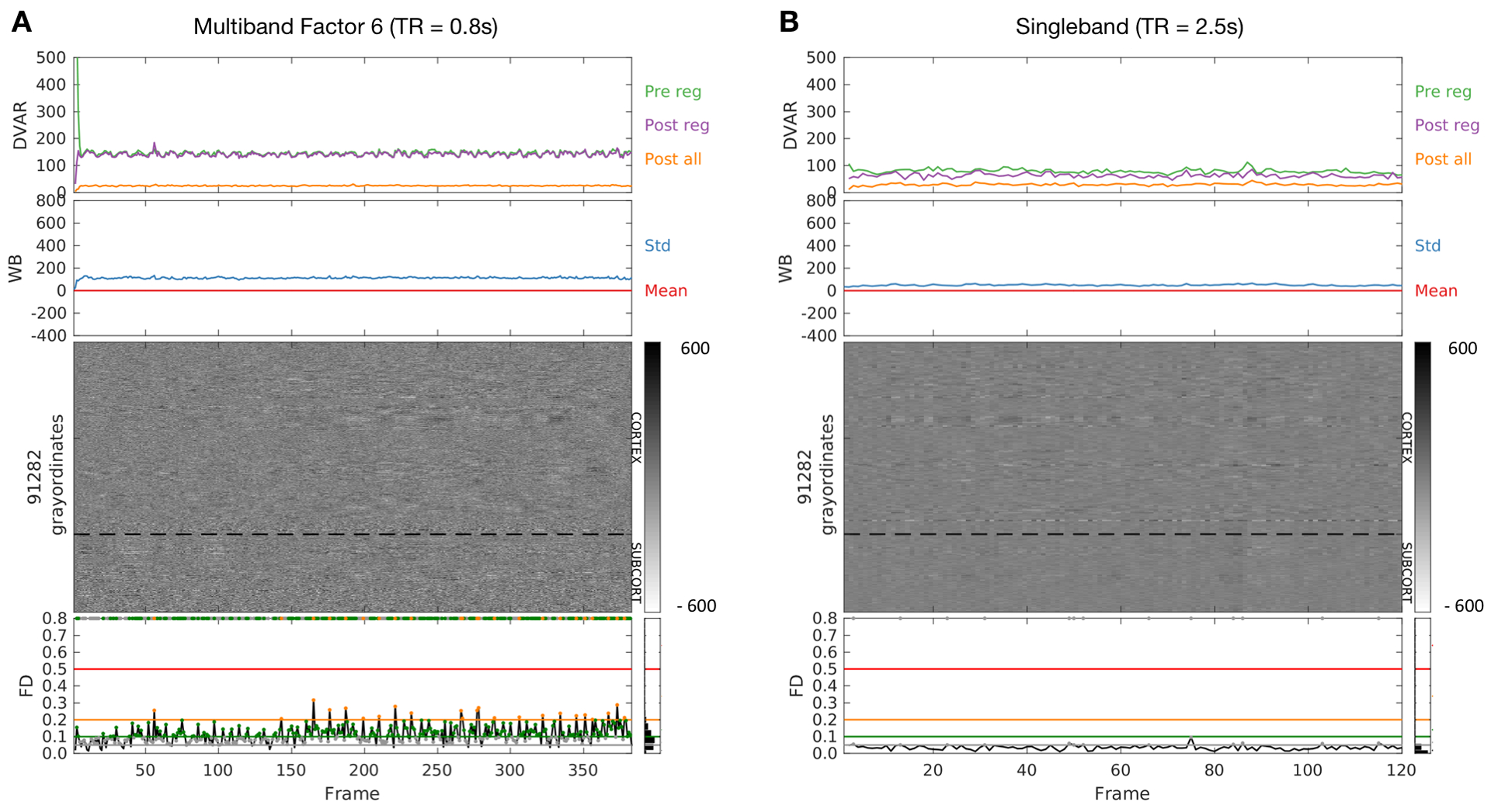
A) One fMRI run acquired with multiband imaging (TR = 0.8 seconds). B) One fMRI run (same subject) acquired with conventional singleband fMRI (TR = 2.5 seconds). 2D voxelwise image intensity plots (gray matter only) represent the time series in voxels or surface data grayordinates as a horizontal stack. This procedure visualizes all the data from a given run (or session via concatenated runs). On top of the 2D grayordinate intensity plots are DVARS measurements (D for derivative of time series, VAR for RMS variance across voxels), prior to denoising (green), post the regression phase (purple), and after the all preprocessing, including filtering (orange). DVARS provides a good estimate of motion that does not rely on retrospective head motion correction (for references, see (Fair et al., 2013; Power et al., 2012; Smyser et al., 2010)). Also included are mean (red) and standard deviation (blue) plots of the whole brain signal. The mean (red) trace is pinned at zero because these plots represent data after processing, which includes whole brain signal regression. On the bottom of the figures, frame displacement (FD) is plotted across the run. Each frame or data point in the FD line plots has a colored circular mark, which represents the FD threshold at which a given frame would have been censored. The corresponding threshold line is displayed as a level. For example, all gray points represent frames that would be excluded at an FD threshold of 0.6 or higher, green points represent an FD threshold of 0.1, orange, FD = 0.2, etc. (illustrative arbitrary thresholds). These points are then duplicated on the upper bound of the graph so that the various thresholds can be easily compared against the grayordinate plots. The idea here is that the proper threshold for removing movement corrupted data should line up with the corrupted data visualized by the 2D grayordinate plot; an example is provided in Figure 4. Pre/Pos reg = Pre/Post regression.

Quantitative assessment of the impact of factitious head motion

The present objective is to assess the impact of factitious head motion on the quality of BOLD fMRI data and to evaluate alternative filtering strategies for mitigating this impact. Our approach to this problem is based on a procedure introduced by Power et al. (Power et al., 2014) for assessing the link between measured FD and fMRI data quality, originally for the purpose of selecting an optimal frame-censoring threshold. This procedure tests the null hypothesis that measured FD is unrelated to data quality. The steps of the procedure for relating FD to fMRI data quality are illustrated in Figure 1. All frames of a given fMRI run are ordered according to increasing FD values. Functional connectivity matrices are computed over sliding windows of 150 volumes (i.e., 1–150, 2–151, …). The mean FC matrix over the first 30 windows (lowest FD) defines a baseline FC matrix. FC matrices are computed over successive windows and their similarity to the baseline is evaluated by correlation of vectorized FC matrices. A relation between FD and fMRI data quality is expected to manifest as a systematic reduction in the correlation between successive windows and the baseline at progressively higher FD values. In the absence of a relation between FD and fMRI data quality, there should be no systematic effect of FD ordering. Thus, the significance of an observed relation can be assessed by comparing the FD-ordered curves to a null distribution generated from surrogate data in which the volumes have been randomly ordered (in our case, 250 permutations). Figure 1 shows a cartoon null distribution of 10 runs for a single subject in black and FD-ordered results in blue. Comparing the true values to the null distribution determines at what FD value the FD-ordered matrices are different from the surrogate data at a given significance (specifically, p < 0.05). In Figure 1, the FD value demarcating the boundary between non-significant (green dot) vs. significant (red dot) FD dependence occurs at about 1.7 mm.

Figure 1. Demonstration of the systematic relation between frame displacement (FD) and functional connectivity (FC).

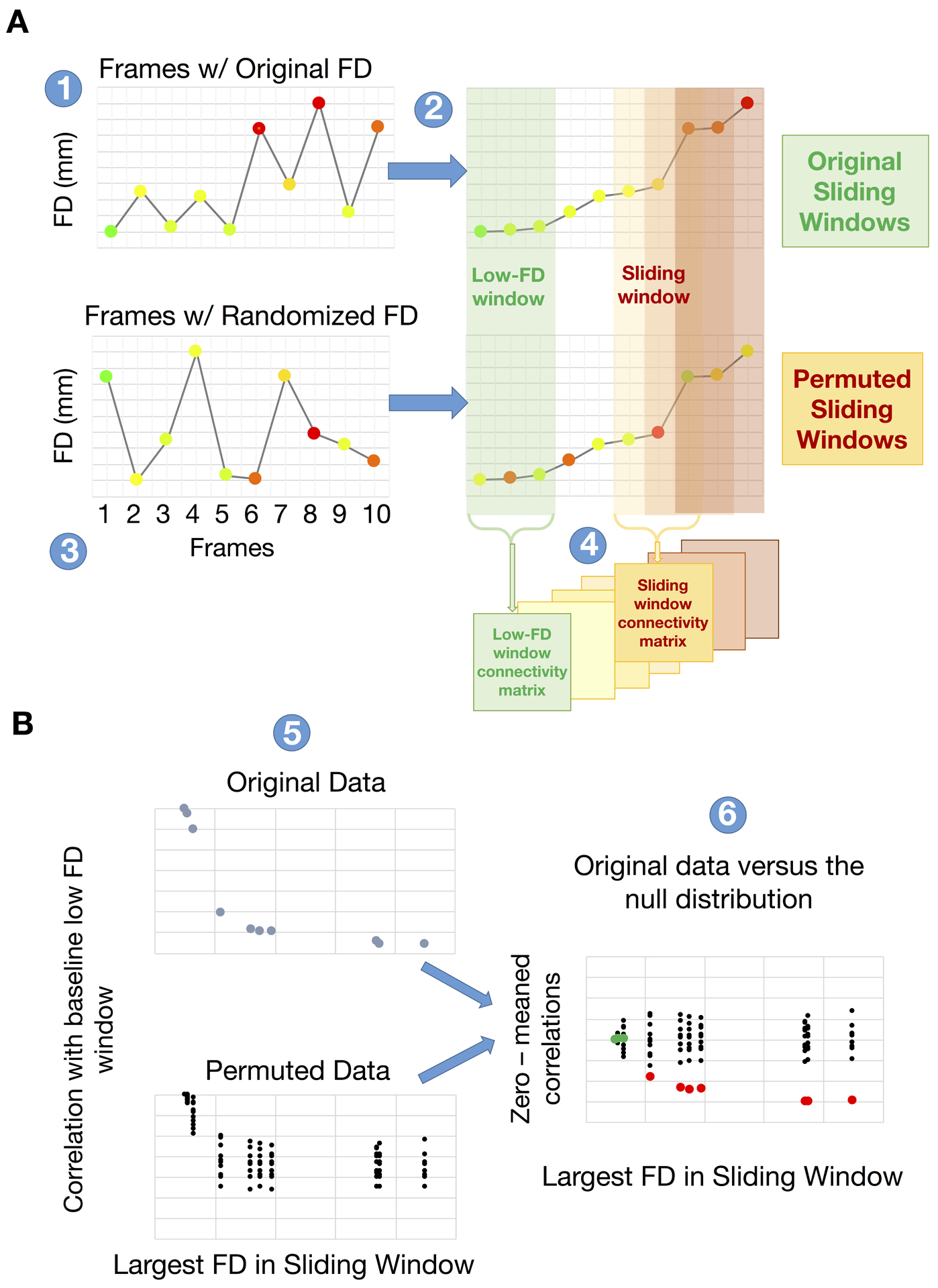
(A) (panel 1) All frames of a given fMRI run are ordered according to increasing FD values (panel 2). Functional connectivity matrices are computed over sliding windows of 150 volumes (i.e., 1–150, 2–151, …). The mean FC over the first 30 windows (lowest FD) defines a baseline FC matrix (green block in panel 2). To evaluate the statistical significance of the FC-FD relation, the frames are randomly reordered (250 permutations) and the procedure is repeated (panel 3). In panel 4, FC in successive windows (31–181, 32–182..) is evaluated and matrix similarity to the baseline FC is computed for both the original and permuted data. (B) A systematic relationship between FD and FC manifests as steadily declining matrix similarity at higher FD windows (blue dots in panel 5, top). The surrogate data generate a null distribution of FC matrix similarity values (black dots in panel 5, bottom). Comparison of FC similarity in the originally ordered windows to the null distribution reveals the FD value at which FC is significantly degraded by head motion (red vs. green dots; panel 6). For simplicity of visualization, the true and null distributions are zero centered.

Figure 2 illustrates how the above-described procedure is used to evaluate alternative strategies for filtering the head motion time series constituting FD_i as defined in Eq. (4). We plot the FD-ordered findings for a single subject against the null (Figure 2A), and then across all subjects (Figure 2B). We then plot the rank of the FD-ordered outcomes across subjects (Figure 2C), and bin these ranks by FD value represented as a heat map (Figure 2D). This procedure provides a vertical distribution of ranks in a FD bin. The cumulative distribution function (CDF) across all FD bins provides an estimate of the average rate at which the windows deviate from the null distribution (Figure 2C,D). If FD is strongly linked to BOLD fMRI data quality, then the shift from randomly distributed ranks occurs at low values of FD. Displacement of this shift towards higher FD values indicates a weaker link between FD and fMRI data quality.

Figure 2. Using the FD sliding window procedure (Fig. 1) to evaluate the success of FD filtering.

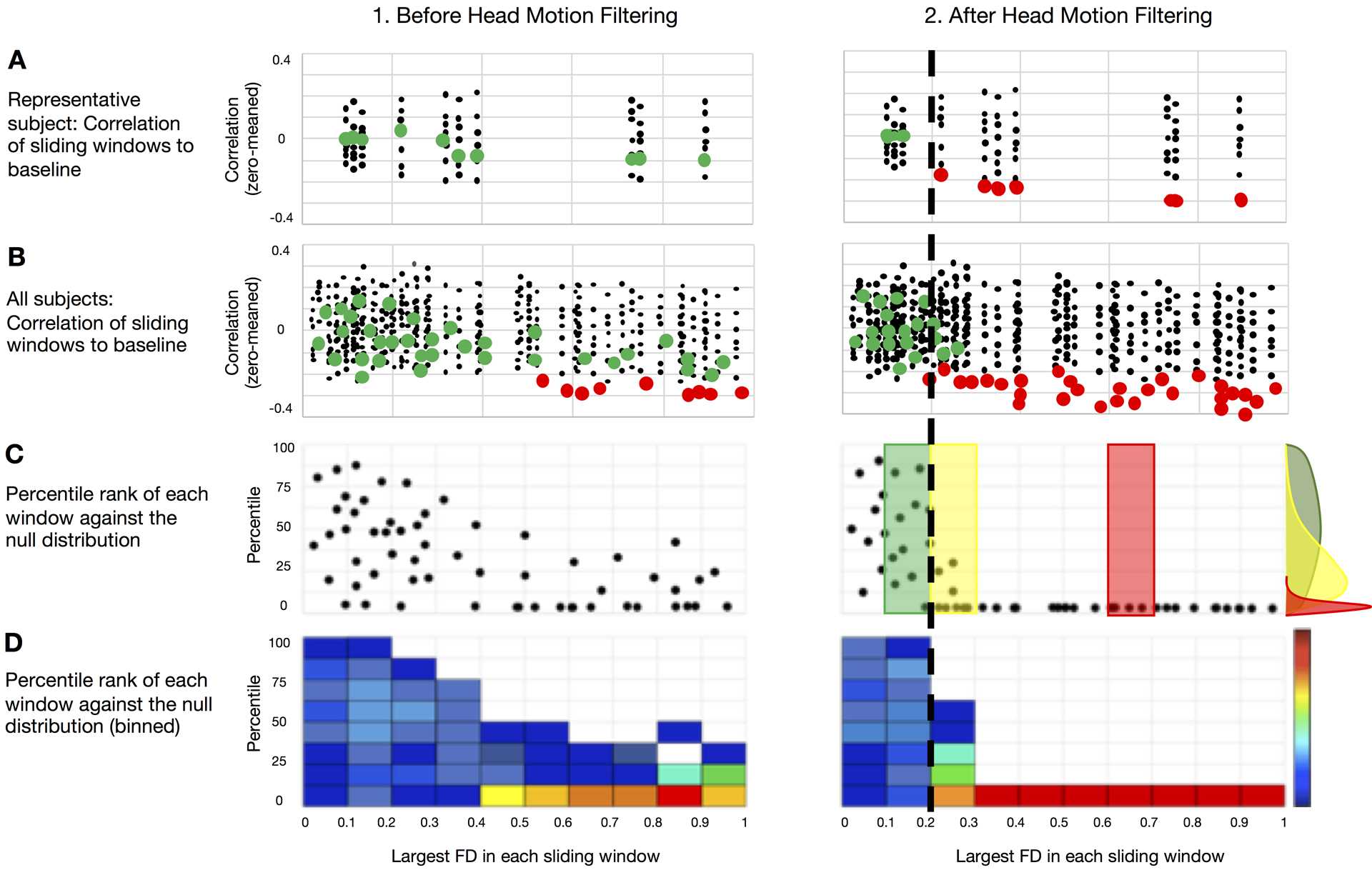
We provide a schematic demonstrating the evalution of the FD sliding window procedure. The objective here is to assess how well FD performs as a measure of data quality. (A) Correlations from the FD sliding windows are compared to the null for each subject for (1.) non-filtered and (2.) filtered FD measurements, colored by significance (green = ns; red = significant). (B) All sliding windows for all participants colored by significance for the unfiltered (1.) and filtered (2.) conditions. (C) Percentage rank (relative to null) of the QC-ordered correlations (from (B)) across subjects, which are binned and represented as a heat map, each dot represents one FD sliding window from one subject. If FD is a good measure of data quality then sliding windows with high FD should poorly match the low FD template, which will be represented in the skew of the distribution of rank orders. (D) Binned representation of (C) as a heat map. The cumulative distribution function (CDF) across all FD bins provides an estimate of the average rate at which the windows deviate from the null model. If the bins deviate from the null model rapidly with increasing FD, it means that FD is a good measure of data quality. The black dotted line represents the approximate level at which FD ordered outcomes deviate from random across individuals (i.e., where the distribution of ranks becomes skewed – illustrated with the colored distributions in (C).

Results

Differences in multiband vs. single band head motion traces

Figure 3 illustrates the manifestations of respiratory motion in FD traces for multiband scanning (TR = 0.8s) and single-shot EPI (TR = 2.5s). The same individual was scanned on the same scanner using both techniques. Breathing was paced at 0.33Hz by a visual cue in both scans (see SI Movie 1). The grayordinate plots and DVARS traces suggest that true head motion in this subject was minimal. Nevertheless, in the multiband data, the FD trace frequently rises above 0.2 mm and exhibits periodicity corresponding to the imposed respiratory pacing. In comparison, in the single band data, the FD trace generally remains below 0.06mm. These qualitative observations demonstrate a fundamental difference in motion estimates provided by multiband data, as compared to single-shot data.

In Figure 4 we show a typical “medium mover” participant in the ABCD study (i.e., a subject randomly selected in the middle quartiles of the distribution). What can be seen in the augmented grayordinate plots for Figure 4A is that large spikes in the movement estimates correspond to artifacts in the data that can be visualized in grayordinate intensity plots, and the other quality measurements: DVARS, whole brain signal, and whole brain signal standard deviations (see black arrows, Figure 4A). These are the same head-motion related BOLD signal artifacts that have previously been documented (Power et al., 2014; Power, 2016). If we take the same motion threshold (FD > 0.2) and examine other places along the FD trace, much of the multiband data that crosses the upper threshold of 0.2, does not appear to have the same types of movement induced artifacts (see red arrows, Figure 4A). These qualitative observations suggest a potential mismatch in movement related artifact and movement in the multiband data.

Figure 4. Augmented 2D grayordinate image intensity plots in a 9-year old ABCD-study participant.

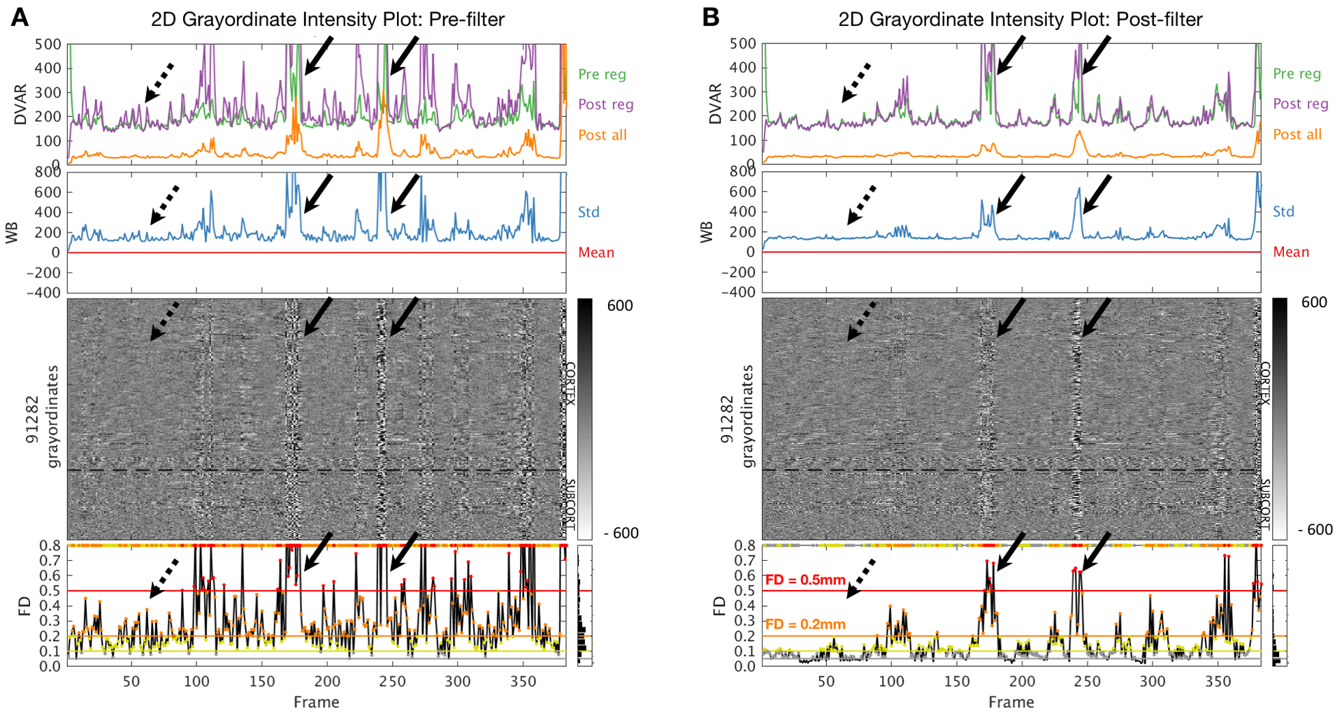
(A) Data processed without motion time series filtering. (B) Data processed with motion time series filtering (FF filter). Black arrows indicate large movement spikes associated with BOLD image artifacts. Motion time series filtering (panel B) removes high-frequency components in the FD trace that exceed censoring thresholds (FD > 0.2 orange; FD > 0.5 red) prior to filtering (panel A). Filtering leaves intact FD spikes associated with image artifact (solid black arrows). Dashed black arrows highlight smaller spikes of apparent motion without associated image artifact. Conventions as in Fig. 3.

Multiband imaging reveals prominent respiratory components in head motion estimates

Having established the possibility of differences in motion estimates for multiband data compared to single band data, we next compared respiratory traces and power spectra of motion estimates in the two data types. Figure 5A illustrates motion parameter time series (3 translations, 3 rotations) together with respiratory belt data acquired in a representative ABCD subject. This subject was scanned with the standard ABCD fMRI protocol (MB 6; TR 800ms). Figure 5A (top row) provides the full trace of a run for a subject, along with brief snapshots of 10 frames of that same run (middle row). We also provide power spectra for those signals (bottom row). A relation between apparent head motion and the respiratory belt is present but not easily perceived in conventional time series plots. This relation is most clearly evident in the power spectral density plots. Chest wall motion is regularly periodic. Accordingly, the respiratory belt power spectrum (gray trace) shows a well-defined peak (at ~0.37 Hz in this participant). This peak is mirrored in the y-translation power spectrum and, to a lesser extent, also in the z-translation power spectrum. While the largest correspondence occurs in y-translation, as would be expected, correspondence in other directions might relate to the fact that the relative head position of the subject often changes from the beginning to the end of a run. It might also represent true head motion related to the respirations themselves.

Figure 5. Frequency domain representation of motion time series in multiband data.

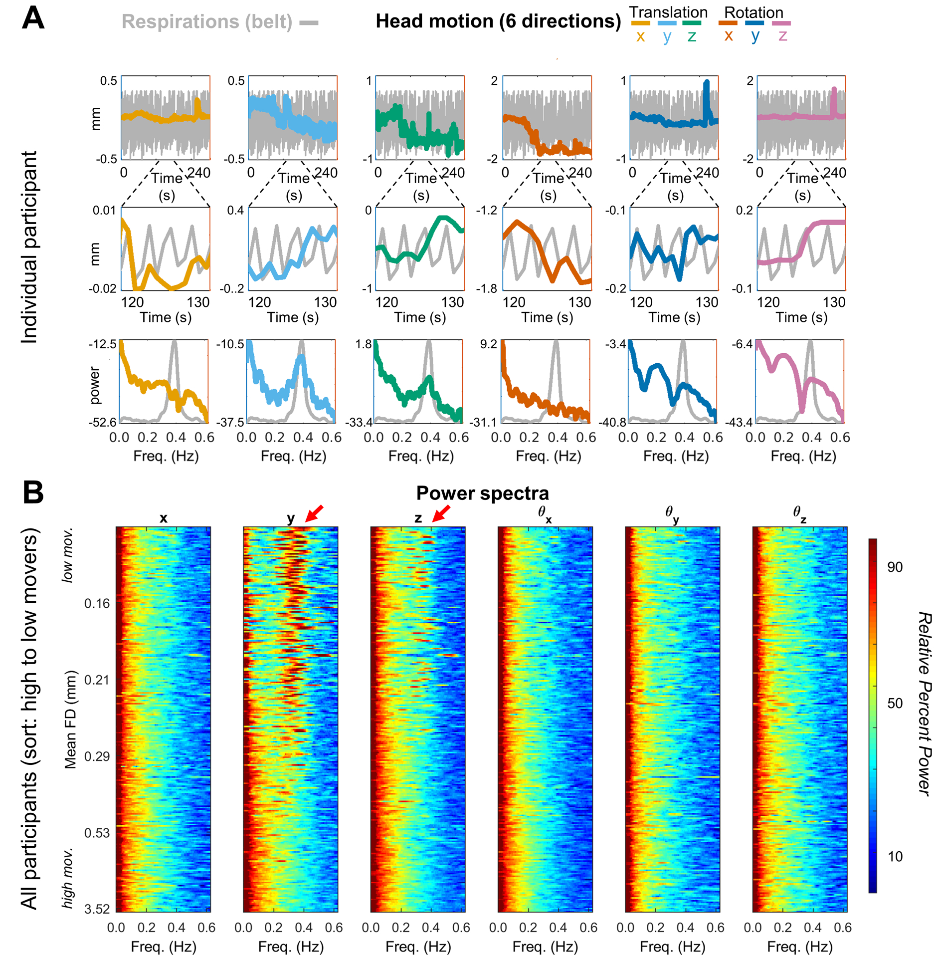
(A) One fMRI run in a single representative ABCD participant (TR = 800 ms). Colored lines represent the translation and rotation motion estimates. Top row: entire (240 s) fMRI run; middle-row: 10 s ‘snapshot’; Bottom row: power spectra of the motion and respiratory belt traces. (B) Power spectra of 62 OHSU ABCD-study participants (mean age 11.6, TR = 0.8s), ordered by mean FD and stacked with lowest movers on top. Red arrows highlight characteristic frequency of respiration artifact (~0.3 Hz). To allow for visual comparisons across a wide range of motion time series power, (i.e., with and without filtering – Fig. 5, Fig. 6 and SI Fig. 2 and 3) the spectra were first represented logarithmically (i.e., in dB) and then Z-scored (details in Appendix B); replication of these figures in one’s own data can be conducted with code provided by github.com/DCAN-Labs. Thus, the respiratory peak is suppressed in very high motion data, which are dominated by low frequency power.

Figure 5B shows motion parameter power spectra in all participants represented as a stack ordered according to total motion (mean FD). The lowest movers are on top. Oscillations at ~0.3 Hz, predominantly in the y-translation parameter, are evident in the lowest movers. Note the absence of low frequency power particularly in the y-translation column (i.e., no evidence of slow head elevations) in low movers. The ~0.3 Hz oscillation becomes progressively less prominent towards the bottom of the stack. This effect arises because the power spectra are normalized (equal total power in all traces). Thus, high motion manifests as a shift of relative power towards low frequencies. In other words, factitious y-translation oscillations, if present, are overwhelmed by true high amplitude head motion. Modest uncertainty regarding the direction of true head motion arises from potential cross-talk between the rigid body parameters represented in Eq. (3). These algebraic complications are detailed in Appendix A.

Respiratory artifact is present, but less prominent in single band data

Figure 6 is identical to Figure 5 except that it shows single-band instead of multiband results. Respiratory belt data were not available in this case. Nevertheless, it is apparent that respiratory artifact occurs primarily in the y (phase encoding) direction. A peak in the power spectrum is present. However, in comparison to the multiband case, this peak is much broader and centered at ~0.14 Hz. Some of this ‘spread’ might be secondary to the interleaved acquisitions where each image is being acquired over a longer TR at a distinct spatial location in time. However, these power spectrum differences between single and multiband data also likely occur because the sampling rate (TR) is not fast enough to capture the true rate of the respirations. Rather, respirations are aliased into other frequencies (see Eq. (5)). This effect is illustrated in SI Figure S1. Any signal that has a frequency higher than half the sampling rate (Nyquist limit) will be detected as a signal of lower frequency. For example, a 2Hz signal sampled at 10Hz will read out at 2Hz. A 5Hz signal sampled a 10Hz, will read out at 5Hz because it is exactly at the Nyquist limit. However, a 6Hz signal sampled at 10Hz, will not read out as 6Hz, but will alias into a lower frequency. In this example, the 6 Hz signal aliases at 4Hz.

Figure 6. Frequency domain representation of motion time series in single band data.

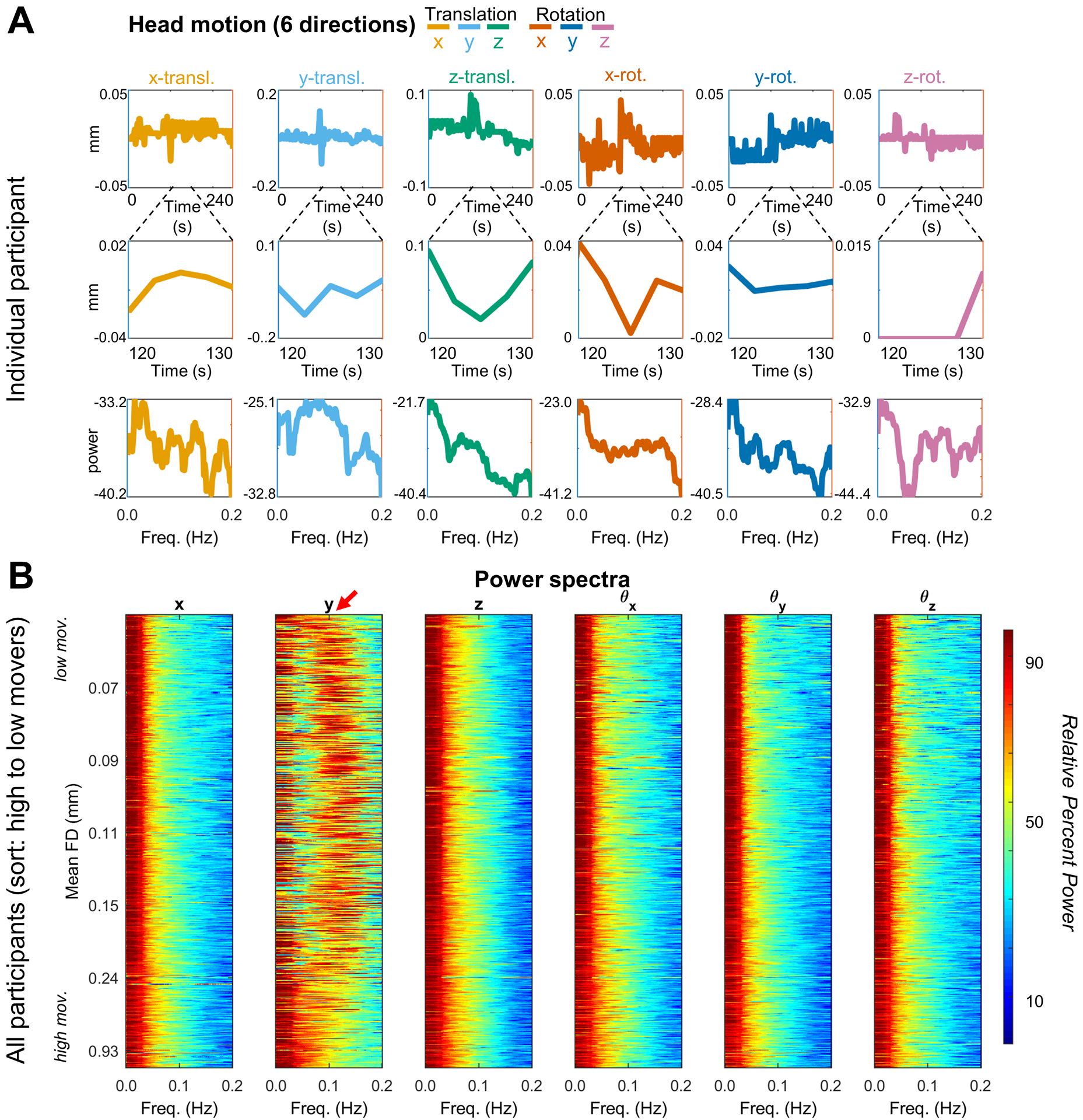
(A) One fMRI run in a single representative participant (TR = 2.5s). All display conventions as in Fig. 5A. (B) Power spectra of 321 OHSU scans (mean age 11.6, TR = 2.5s), ordered by mean FD and stacked with lowest movers on top. Red arrow highlights respiration artifact. As in Fig. 5B the spectra were first represented logarithmically (i.e., in dB) and then Z-scored (Appendix B). The respiratory spectral peak (presumed true center frequency ~0.3 Hz) is both comparatively broad in relation to the resolved spectral range (Nyquist folding frequency = 0.2 Hz) and aliased to ~0.1 Hz = 0.2 - |~0.3 – 0.2| Hz.

In SI Figure S1 we provide an illustration of what frequencies might be expected for a given respiratory rate and for a given sampling rate (TR). Three examples are given for 15, 20, and 25 breaths per minute. What is shown is that the artifact in the motion traces for a TR of 800ms (or 0.8s) will match the true respiratory rate of a given participant; however, for slower TRs (single-band data) the respiratory rate will be aliased into different frequencies. Thus, any variation in respiratory rate during a scan is likely to be spread into different frequencies, broadening the spectral peak (see Figure 6B – red arrow, relative to Figure 5B – red arrow). This mismatch between true respiratory rate and what can be observed in motion traces might be one reason why these artifacts were initially overlooked in single-band data.

An experimental demonstration of the above-described effects is presented in Figure 7. Resting state fMRI was acquired in single subject while breathing was visually paced at exactly 0.33 Hz (see supplementary movie to view the pacing display). The identical multiband sequence was run at TR = 0.8, 1.5, and 2 seconds. fMRI was collected also using a single-shot sequence at TR = 2.5 s. Aliasing of the respiratory signals in Fig. 7A–D closely matches the theory expressed in Eq. (5) and illustrated in Fig. 7E. Note also that the respiratory peak is narrow because it was precisely paced.

Figure 7. Respiratory artifact aliasing as a function of sampling rate.

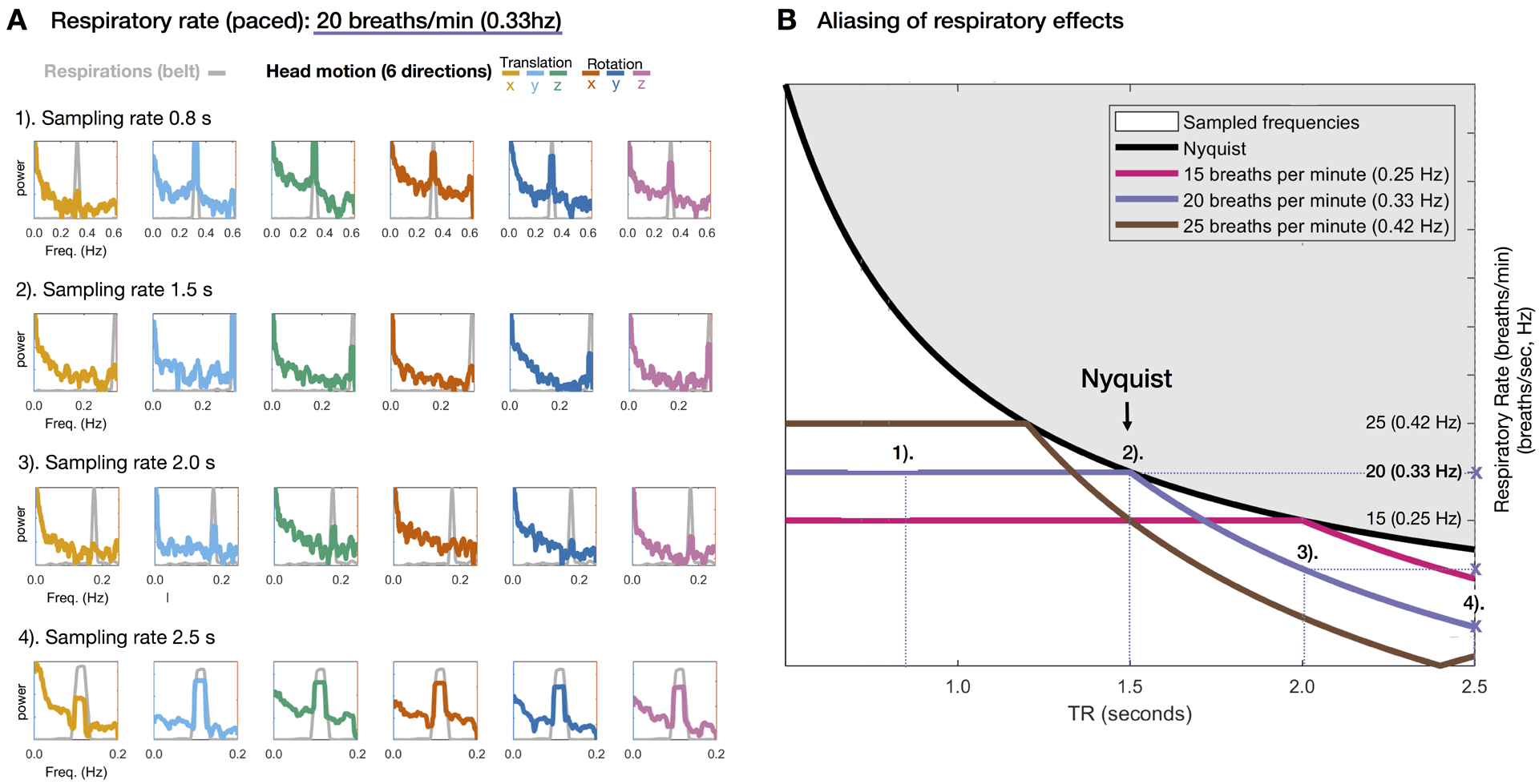
(A) BOLD data were collected while the participant’s respiratory rate was visually paced at exactly 0.33Hz (20 breaths/min; see Supplementary Movie 1) at TRs of 1). 0.8 s (multiband), 2). 1.5 s (multiband), 3). 2.0 s (multiband) and 4.) 2.5 s (singleband). The respiratory belt data were sampled at the same rate as the BOLD data for each TR (e.g. for a TR of 2.0 s, respiration data (gray) were sampled every 2.0 s). Note that the peak power for the respiration (gray) and head motion traces (6 directions) overlap closely and are moved to lower frequencies by sampling at larger intervals (1 – 4). (B) Superimposition of empirical spectral peak values over predicted values based on Nyquist theory as outlined in Methods. For sampling rates of 1). 0.8 s and 2). 1.5 s there is no aliasing and the respiratory peak stays at 0.3 Hz. For sampling rates of 3). 2.0 s and 4). 2.5 s the respitarory peak gets aliased to lower frequencies (marked by purple ‘X’). Note close match of empirical (A) vs. theoretical (B) spectral peak frequencies.

Respiratory artifacts change with phase encoding direction

It could be argued, despite the evidence presented thus far, that the respiratory artifacts demonstrated here are purely mechanical (SI Figure 5). In other words, true respiratory motion can be transmitted from the chest to the head by mechanical linkage through the neck, as discussed above in connection with Fig. 5. Such motion is most likely to occur as z-direction displacement (as in Figs. 5 and 6) or rotation about the ear-to-ear axis (θ_x; pitch). If true, this motion may generate BOLD signal artifact on the basis of spin history effects (Friston et al., 1996) and changes in B₀ due to motion (movement through non-uniform field/shim) unrelated to repiratory-related Bo changes (or drifts). To show that the additional motion related findings secondary to B₀ are distinct, we obtained data in a second participant who is known to be a very low mover. We then collected several additional BOLD runs in which the phase encode direction varied. The participant was blind to this manipulation. Figure 8 shows spectral analysis of motion trajectories obtained in four of these runs (see also Figures S2 – S4). The respiratory artifact in the motion traces clearly follows the phase encode (PE) direction (i.e., y-translation to x-translation or vice versa). Respiratory power is also present in other directions. Respiratory power not in the phase encode direction most likely reflects true brain motion, with some evidence in the traces that this true respiration related motion may also be leaking into other directions (see Discussion and Appendix A). Our finding of B₀ artifact at the primary respiratory frequency is also clearly visualized with Human Connectome Project (HCP) data (for processing details see (Miranda-Dominguez et al., 2018)). whose phase encode direction was LR/RL as opposed to ABCD data, which was AP (SI Figure 5). Interestingly, in the Human Connectome Data additional artifacts of unknown origin, restricted to the phase encoding direction, are seen in the same narrow frequency band across most subjects, both at a higher frequency (~0.57 Hz), as well as a lower frequency (~0.16 Hz) (SI Figure 5). Overall, these results show that respiratory artifact in the phase encode direction is induced by B₀ perturbations. Thus, the component of head motion that moves with the phase encoding direction is factitious while other components of respiration related head motion are real, with potential ‘leakage’ of the B₀ artifact into other directions.

Figure 8. Dependence of factitious respiratory motion on phase encoding direction.

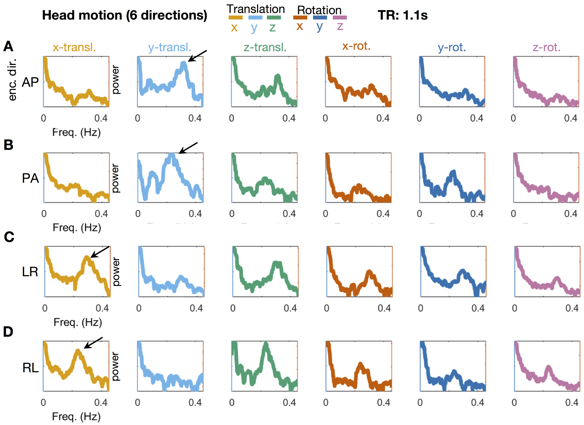
To show that motion related findings secondary to B₀ are distinct from true brain motion, we obtained additional data in a single participant known to be a very low mover. Four BOLD fMRI runs (TR = 1.1s) were acquired with phase-encoding (PE) directions AP, PA, LR, RL. The participant was blind to PE condition. (Additional data acquired in a separate session with distinct scan parameters are shown in SI Figures S2–S4). Note principal respiration peak (~0.23 Hz; black arrows) in the motion parameter capturing translation in the PE direction: y-translation for AP and PA (Panels A and B) and x-translation for LR and (panels C and D). This effect is highly consistent with factitious head motion induced by B₀ modulation. ~0.23 Hz signals largely invariant with respect to PE direction occur in the z-translation and x-rotation parameters. These signals most likely represent true translation along the long body axis and head nod about the ear-ear axis arising from mechanical linkage of the head to the chest through the neck. Respiratory motion in other parameters (y-rotation, z-rotation) could represent true head motion or “leakage” (see Appendix A).

Filtering FD data corrects for respiratory artifacts and improves estimates of data quality

Having established the factitious effects of respirations on motion estimates, we then turned our attention to reducing them. To correct head motion estimates for respiration related B₀ artifact, we applied a bandstop/notch filter to the rigid body alignment parameters [Eq. (3)]. Two filter strategies were evaluated. First, we evaluated a generic, Fixed Frequency [FF] filter designed to exclude a range of respiratory rates (see Methods). The FF approach does not require respiratory rate measurement in individuals. In the second approach, we used respiratory belt data (see Methods) to generate individually tailored filter parameters (Subject-specific Frequency [SF] filter). The effects of applying the FF filter are shown in Figure 4B.

Marked improvement in the linkage between FD and functional connectivity data quality (gray ordinates block) is evident on comparison of Figures 4A vs. 4B (black arrows). The impact of this improvement on FD-based frame censoring is dramatic. Thus, assuming a censoring criterion of > 0.2 mm (orange line in FD trace), very few frames would survive without filtering (panel A). In contrast, with filtering (panel B), censored frames align more strongly with the artifact.

The DVARS trace also improved post filtering. The reason for this improvement is that regression of factitious head motion waveforms introduces spurious variance. Thus, main field (B₀) perturbations caused by chest wall motion may indirectly corrupt fMRI data via distorted nuisance regressors. This effect is independent of frame censoring. Hence, there are reasons to remove factitious components from motion regressors even if frame censoring is not part of the analysis strategy.

Supplementary Figure 6 and Supplementary Figure 7 provide replicates of Figure 5 after FF and SF FD filtering, respectively. These figures illustrate the aligment of the filter with the respiration-induced artifact. A close look at both Supplementary Figure 6B (FF filter) and Supplementary Figure 7B (SF filter) shows that both these methods do not perfectly capture the artifact. Indeed, in Supplementary Figure 7B, particularly for high moving subjects (i.e., bottom of graph), the filter impinges on true motion values. In other words, the identification of the dominant respiratory rhythm in high movers is difficult. So, the SF filter might be more precise for some individuals, but less so for others, as compared to the FF filter. For this reason the overall performance of both of the SF and FF filter are largely similar (Figure S8E).

Filtering head motion estimates improves data quality

To quantify the impact of filtering motion parameters on BOLD data quality, we used FD sliding window methodology introduced by Power et al., (2014). The FD sliding window method was originally used to select the frame-censoring criterion using a rational procedure. Here, we adapt the FD sliding window approach to assess the fidelity of a quality assurance measure, specifically, FD, as outlined in Figures 1 and 2 (see Methods).

Results obtained with the FD sliding window procedure are shown in Figure 9 and SI Figure S8. The basic result is that filtering causes the boundary between “low” vs. “high” quality data to shift towards lower FD values. In other words, without filtering, relatively high FD values do not reliably indicate compromised data quality. The unfiltered FD measurements are more random than FD measurements that have been filtered using the FF filter (or SF filter – see Supplementary Figure S8). The top row of Figure 9A demonstrates this effect in a single subject, where fewer green points (windows similar to the baseline) extend up to the highest FD values. In contrast, with FF filtering (Fig. 9A), a clear boundary between “low” vs. “high” quality data (sharp transition from green to red points) occurs at 0.26 mm. Figure 9B plots the rank of the FD-ordered results across subjects (as in Figure 2B). Figure 9C bins those ranks (as in Figure 2C). These plots include all subjects and represent a vertical distribution of ranks (relative to randomly ordered volumes) of sliding window comparisons to the baseline. The cumulative distribution function (CDF) across all FD bins (Figure 9C,D) estimates the average rate at which the windows deviate from the null model (as in Figure 2B,C). Filtering causes the CDF to shift leftwards. This leftward shift reflects, at the population level, better correspondence between FD and data quality, as described above in individuals. Figure 9E plots the CDFs obtained in the FF filter versus the ‘no filter’ conditions. The FF filter CDF significantly differed from the ‘no filter’ CDF (p< 0.0001) by the Kolmogorov–Smirnov (K-S) test. Similar CDF findings were obtained with the SF filter (see Supplementary Figure 8). Also see Supplementary Figure 9, which provides an alternative approach to measuring the significance of this effect, as well as, SI text which describes how the reliability of connectivity measurements improves with the filter condition (SI Figures 10 & 11).

Figure 9. Demonstration that motion parameter filtering enhances the link between FD and FC.

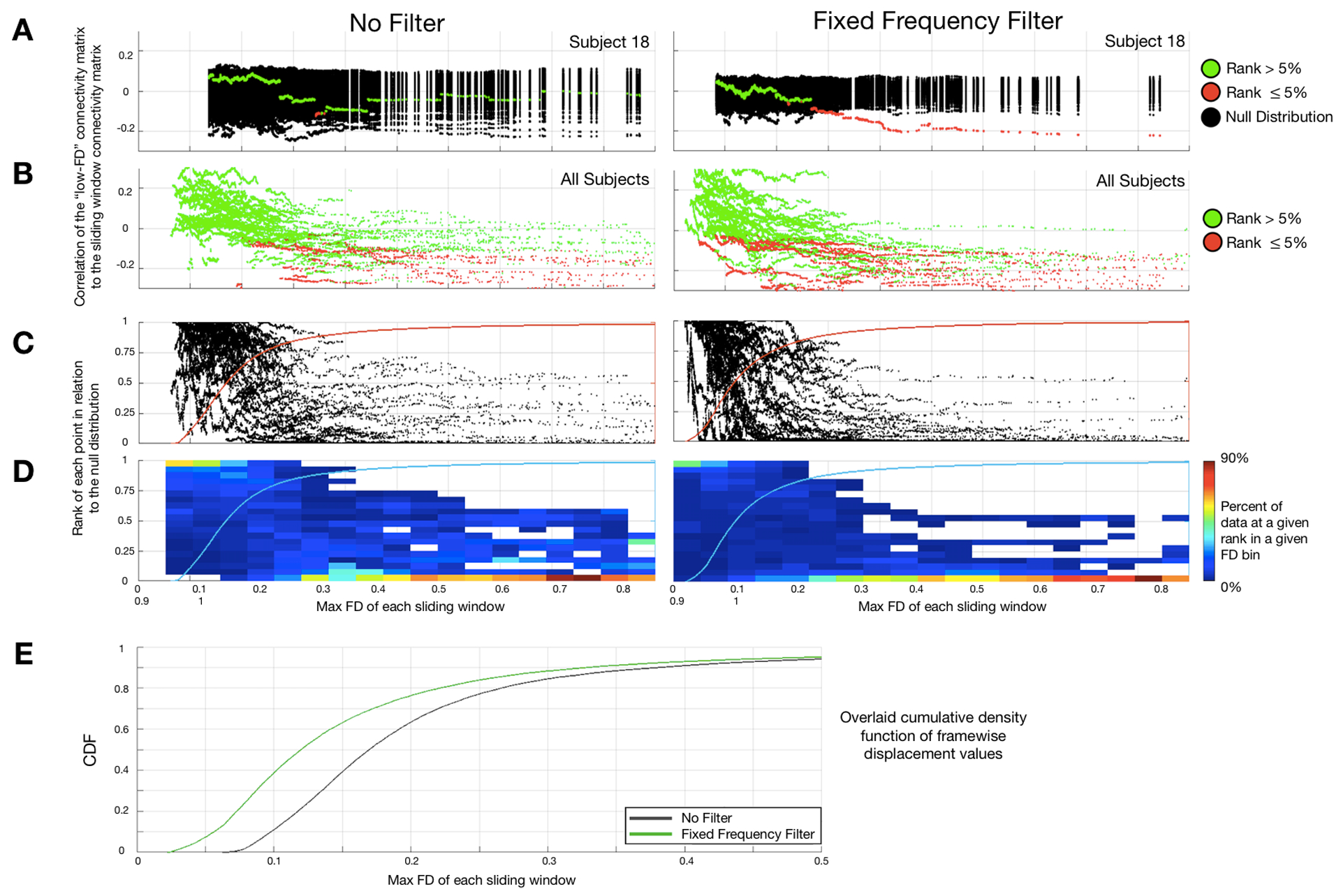
This figure follows the logic illustrated in Fig. 2. “No-filter” and Fixed Frequency (FF) filter results are shown on the left and right, respectively. (A) Single participant results. Values in red are significantly different from random; values in green do not significantly differ from random. (As in Fig. 2, the true and null distributions are zero centered). Thus, absent motion parameter filtering, there is little relation between FD and FC. (B) Significance of all FD:FC associations for all subjects. Motion parameter filtering causes the appearance of a significant FD:FC relation to appear at lower rank-ordered FD values (8^th %-tile vs. 20^th %-tile). (C) Percentage rank (relative to null) of the FD-ordered FC outcomes across subjects. (D) Binned heat map as in Fig. 2D. (E) Cumulative distribution functions (CDFs) for the filter and ‘no filter’ results. These CDFs provide an estimate of the average rate at which windowed FC deviates from the null model. Filtering shifts the CDF to the left (green trace), i.e., improves the link between FC and motion estimation. This effect is statistically significant (p< 0.0001, Kolmogorov–Smirnov (KS) test applied to the two CDFs). See SI Figure 4 for similar results obtained with the SF filter.

Reliability of connectivity measurements improves with filtering of FD values

Two additional tests were conducted to examine the reliability of our connectivity measurements with and without FD filtering. First we applied a split half replication procedure whereby we randomly compared two separate runs within an individual and then correlated connectivity matrices of these split halves across a series of FD thresholds. This procedure was performed for both the FF and no filter conditions (SI Figure 10). Second, we searched for correspondence in correlation matrices when using DVARS or FD criteria for censoring data frames (with and without filtering), the idea being that the FD frame censoring approach (FD filtering vs. no FD filtering) that captures the most head motion artifacts would most closely resemble correlation matrices obtained when frame-censoring using DVARS measurements (SI Figure 11). Split half reliability of the processed data was improved by the FF filter (see SI Figure 10). In addition, frame-censoring with filtered FD values (FF) increased the similarity with functional connectivity data frame-censored using a DVARS criterion (SI Figure 11).

Real-time implementation of head motion filtering in FIRMM software

Real-time motion monitoring tools such as FIRMM can reduce costs and improve data quality. To improve the accuracy of real-time head motion estimates, filtering of respiratory frequencies has been built into version 3 of FIRMM software. Scanner operators have the option to apply the FF filter in real time (Figure 10 and SI Movie 2) via a GUI that provides users with control over filter parameters. This type of control is necessary because different subject populations (e.g., children vs. adults) may have different respiratory rates. Figure 9 shows the FIRMM display for unfiltered and filtered FD data acquired in three 5-minute resting state BOLD fMRI runs. As in our original report (Dosenbach et al, 2017), on-line filtered FD values very closely track filtered FD values generated by the off-line processing stream (Figure 10 C,D).

Figure 10. On-line (FIRMM) vs. off-line motion censoring.

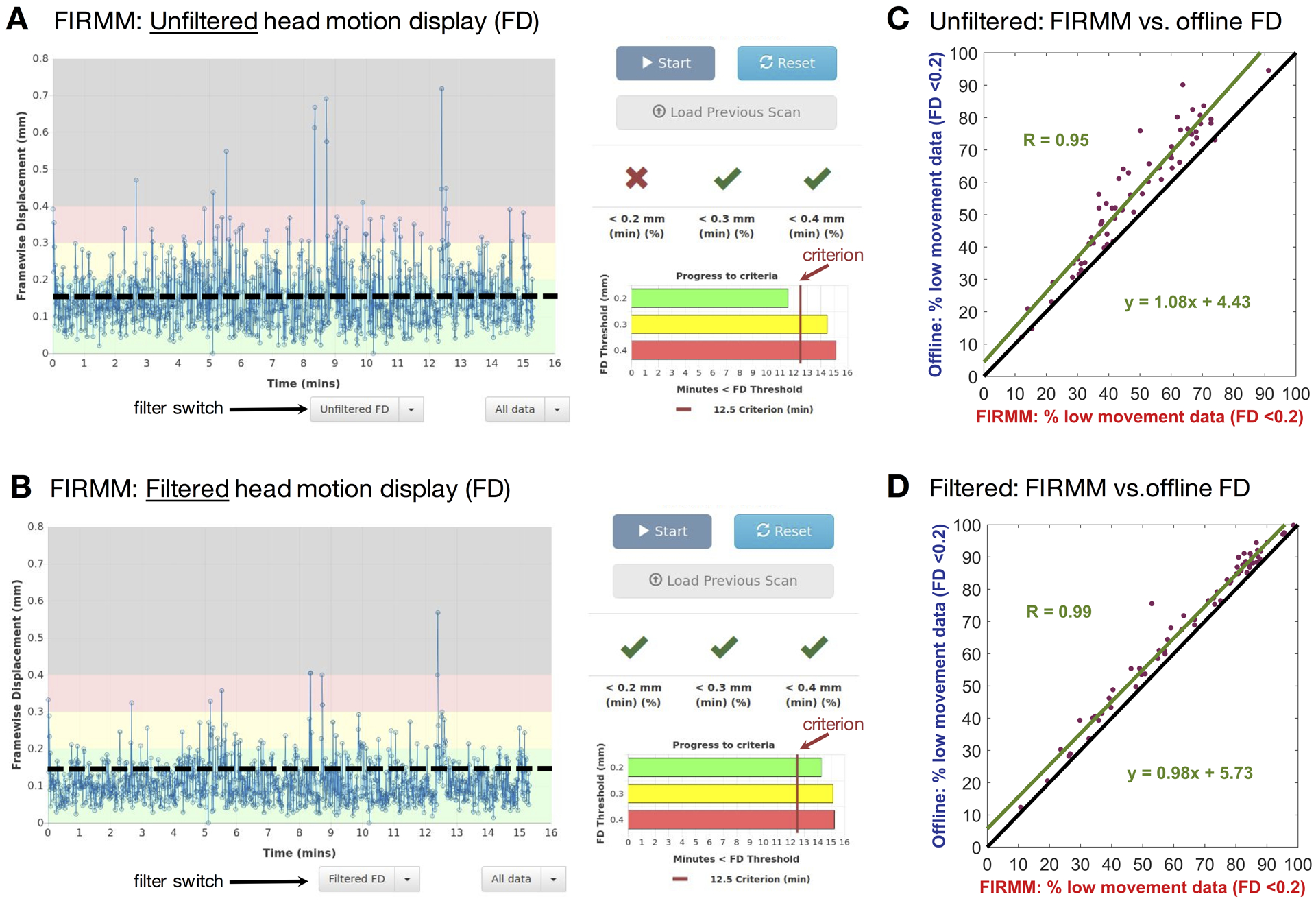
(A) FD computed without filtering for 3 × 5-minute resting state runs acquired in one participant with. (B) Same with filtering. (C) For all participants, percentage of usable frames determined on-line by FIRMM compared to post-processing (mcflirt). (D) Same with filtering. Note strong correspondence between the on-line and off-line results. FIRMM rejected slightly more (~5% of total) frames. In panels C and D, the line of identity is heavy black.

Discussion

We show that respiratory motion can artifactually inflate head motion estimates, causing overly aggressive frame-censoring and unnecessary data loss. Faulty head motion estimation also interferes with other denoising techniques besides frame-censoring. Specifically, corruption of nuisance regressors derived from retrospective head motion correction introduces spurious variance into the fMRI time series. This spurious variance appears in DVARS time series and is reduced by appropriate head motion filtering (Fig. 4). Similar logic underlies the rationale for adjusting the spectral content of head motion time series prior to their use as nuisance regressors (Carp, 2011; Hallquist et al., 2013). For this reason our filter is applied to translation and rotation values after they are estimated and utilized for the remainder of the processing. We demonstrate these principles using on-line as well as off-line head motion estimation based on registration of reconstructed images. However, the same issue potentially arises with any motion estimation strategy. For example, volumetric navigator sequences for structural MRI, which adjust acquisition parameters based on head motion estimates between whole-brain EPI snapshots, might overcorrect during low-movement scans (Zaitsev et al., 2017). To address these important concerns, we evaluated a notch filter that drastically reduces the effects of respirations on FD estimates and thus improves MRI quality. Finally, we demonstrate near real time implementation of on-line motion estimation including notch filter correction of FD estimates. This development represents an important improvement of our existing real-time motion monitoring software (FIRMM).

Distribution of respiratory motion across rigid body parameters

Although respiratory head motion, to a large degree, is likely factitious in origin and most prominently occurs in the phase encoding direction (Figs. 5,6,8), head motion at the same frequency may also appear in any motion parameter, albeit to a lesser extent (e.g., Figs. 8, S2 – S4). Indeed, since the release of our pre-print (Fair et al., 2018) similar findings have now been replicated elsewhere (Power et al., 2019). Respiratory head motion affecting parameters other than phase encoding direction displacement can arise on the basis of a few distinct mechanisms that must be distinguished in future work. First, the data we used were acquired with slices aligned along the anterior-posterior commissure, which is a tilt of ~15 deg from axial. This positioning would cause the phase encoding gradient to be mainly in y, but with a z component, which might explain the secondary, but lesser, effects we see in the z-direction. Second, true respiratory motion can be transmitted from the chest to the head by mechanical linkage through the neck, as discussed above in connection with Fig. 5. This motion is most likely to occur as z-direction displacement (as in Figs. 5,6,8) or rotation about the ear-to-ear axis (θ_x; pitch). Being true motion, it would generate BOLD signal artifact on the basis of spin history effects (Friston et al., 1996). Third, factitious head motion may appear in any motion parameters owing to algebraic cross-talk (see Appendix A for details) or a repositioning of the head relative to the original reference frame. In this case, the artifact would appear to ‘bleed’ or ‘leak’ into the other directions. It is for this reason we chose to apply our notch filter to all directions of head motion. In short, it is likely that the presence of factitious head motion accounts for some of the correspondence between motion estimitates and respirations (Power et al., 2017). However, respirations contaminate BOLD data in multiple ways (Birn et al., 2006; Power et al., 2017), and as such, additional work is needed to more fully disentangle these complex issues.

Pros and cons of Fixed Frequency (FF) and Subject Specific (SF) FD filters

We empirically designed the FF notch filter to capture a large proportion of respiratory frequencies in the ABCD participant sample (see Methods). This filter worked well in improving the reliability of functional connectivity data. However, since different populations and age groups have different respiratory rates (Wallis et al., 2005), the FF filter should be tailored to the population under study. Such tailoring could also take into consideration respiratory variability within individuals, which manifests in the power spectra as a wider artifact peak (as shown in Figure 5 as compared to Figure 7). The filter parameters chosen for the ABCD population are unlikely to be appropriate for all populations. Accordingly, the FIRMM software enables the user to modify the FF filter parameters via the GUI. Some populations might not require motion parameter filtering at all. For example, infant chest excursions are likely only to minimally perturb the main field. For this reason, FIRMM allows the user to control whether filtering is enabled or disabled. To aid in such decisions, we have released software in our repositories (FIRMM, 2017), which will recreate the extant images in Figure 5, and allow investigators to visualize the artifact in their own data, and allow for appropriate thresholding.

In principle, the SF filter strategy, which matches the filter characteristics to each individual’s respiratory rate, should be more accurate in eliminating factitious components from the head motion regressors. In the current results, the SF filter performed similarly to the FF filter in low movers. In high movers, the SF filter strategy often failed to correctly identify the respiratory component (Supplementary Figure 7). Thus, while the SF filter is appealing, there are methodological pitfalls. First, not all studies collect respiratory belt data, which is required for using a SF filter. Second, even if respiratory data were collected on a subject, they could be inaccurate. Often the respiratory belts are not fit properly or become dislodged during scanning. Along the same lines, identifying the peak respirations from the motion numbers themselves can also be problematic, as noted above. Future work is needed to develop reliable SF filtering. One option might simply be to modify the notch filter applied here to a low-pass filter where identifying the proper range of threshold would not be required (Siegel et al. 2017). Until work optimizing the SF approach is conducted, our current recommendation would be to utilize a filter that is general and consistent across participants.

In this manuscript we do not make specific recommendations for adjusting FD frame censoring thresholds to account for the effects of FD filtering. Applying either the FF or SF filter necessarily reduces overall power of the FD traces. This reduction in power likely requires a revisiting of the thresholds for frame censoring that have become common practice (e.g., FD < 0.2) (Power et al., 2014). While beyond the scope of the current report, a systematic evaluation to this end is needed in future work (e.g., other types of filters, such as ICA, might improve on current methods). Importantly, as noted by Power and colleagues (Power et al., 2014), all datasets, with or without filter adjustments, should be evaluated independently for proper FD thresholds.

FIRMM allows adapting the FD filter parameters to the study population

FIRMM was initially created as a response to difficulties in collecting sufficient quality ‘low movement’ data for t-fMRI and rs-fcMRI studies. FIRMM calculates and displays curated motion values (i.e., frame displacement [FD]) and summary statistics during data acquisition in real time, providing investigators and operators estimates of head motion data. The benefits of using FIRMM to reduce costs and improve data quality have been thoroughly examined in prior reports (Dosenbach et al., 2017; Greene et al., 2018). Importantly, FIRMM and other real-time motion estimators rely on accurate translation and rotation numbers. The implementation of the notch filter in real time (see methods for our approach) improves the accuracy of the motion values in FIRMM.

There are a few considerations for FIRMM users, when applying our FIRMM notch filter to the motion estimates (see Methods). The filter recursively weights the two previous samples to provide an instantaneous filtered signal, and thus cannot start until the third sample. In addition, to avoid a phase delay with respect to the original signal, the filter is applied again in the reverse direction (cancelling the phase delay). In real time, this requires waiting until the 5^th sample to provide a best estimate of filtered motion for the third data frame. Each time a new frame arrives the process is reapplied to all frames available, continually converging closer to the optimal output obtained when the filter is applied twice to the entire sequence (as in post-processing). This filtering procedure works well and only leads to a small delay in motion estimates of at least two frames. For a large majority of users this small delay for fast TRs (< 1 sec/frame) accompanying multiband imaging is non-consequential. Nevertheless, alternative real-time filtering algorithms exist that theoretically could reduce or eliminate this delay (Glover Jr, 1977). Implementation of real-time filters without any delay will be considered in the future.

Respiratory artifacts in motion estimates are not isolated to multiband sequences

Although it has been known for over a decade that respiratory motion perturbs the main field (Van de Moortele et al., 2002) these effects have gone largely ignored. Several previous methods have been presented that attempt to address this issue by measuring the frequency shift due to respiration using short navigator acquisitions, and correcting it retrospectively (Barry and Menon, 2005; Pfeuffer et al., 2002; Thesen et al., 2003; Wowk et al., 1997) and prospectively (Benner et al., 2006). All of the sequences evaluated in this study included these features, both prospectively adjusting the center frequency for each slice or slice-group (Benner et al., 2006) and retrospectively adjusting the phase of measured k-space data (Pfeuffer et al., 2002) using the additional phase information in the N/2 ghost navigator (Thesen et al., 2003). Thus, the respiration-correlated effects we observe are the residuals after these on-scanner corrections. Clearly, despite the on-scanner correction, significant residual errors remain in the BOLD timeseries. These effects materially compromise denoising strategies, especially with SMS sequences (e.g., Fig. 4). As fast fMRI with SMS sequences becomes the standard of practice, large, ongoing, multi-site projects, such as Adolescent Brain Cognitive Development (ABCD), must consider this issue. Here, we demonstrate one approach for managing factitious head motion due to respiratory perturbations of the magnetic field (B₀).

Similar corruption of head motion estimates in single-band data has not been widely recognized. Reasons for this circumstance include that frequency aliasing (Figures 7 and S1) disguises the source of the problem and that respiratory rate variation normally spans a comparatively large fraction of the resolvable spectral band (Figure 6). However, factitious respiratory motion artifact can be detected in single-band data. Although we did not systematically examine the effects of applying our notch filter to single band data, doing so might improve previously obtained results. We note that this may not be straightforward as aliasing [(Eq (5)] must be taken into account. As noted above, one option, might be to simply apply a low-pass filter, instead of a band-stop or notch filter (Gordon et al., 2017; Gratton et al., 2018; Laumann et al., 2016).

Conclusions:

Properly controlling for motion artifacts in fMRI is of the utmost importance in both clinical and research applications. The current report shows that main field (B₀) perturbations generated by chest wall motion corrupt head motion estimates. Factitious head motion leads to the false appearance of compromised data quality and introduces spurious variance into fMRI time series via corrupted nuisance regressors. These effects are readily apparent in SMS sequences but are also present in single-band sequences. Notch filtering tailored to the respiratory frequency band improves the accuracy of head motion estimates and improves functional connectivity analyses. Notch filtering can be applied off-line during post-processing as well as on-line to improve real-time motion monitoring. Additional work is needed to improve strategies for fine tuning filters to better match individual respiratory rates.

Supplementary Material

Supplementary Figure 1

Supplementary Figure 1. Frequency aliasing. Oscillatory activity faster than the Nyquist folding frequency 1/(2TR)) aliases to lower frequencies, as described by main text Eq. 5. This frequency aliasing effect is illustrated at TRs of 0.72 s (A), 0.8 s (B), 2.0 s (C) and 2.5 s (D) for respiratory rates (breaths per minute) of 15 (green circles), 20 (orange circles) and 25 (purple circles).

Supplementary Figure 2

Supplementary Figure 2. Dependence of factitious respiratory motion on phase encoding direction. This figure parallels main text Fig. 8. The fMRI sequence (ABCD) is different and the TR (= 0.8s) is somewhat shorter. As in Fig. 8, respiratory factitious motion depends on the phase encode direction: y-translation for AP and PA (Panels A and B) and x-translation for LR and RL (panels C and D). The other four motion parameters reflect varying quantities of respiratory motion that most likely is real with some contribution from “leakage” (see Appendix A).

Supplementary Figure 3

Supplementary Figure 3. Dependence of factitious respiratory motion on phase encoding direction. This figure parallels main text Fig. 8 and is identical to Fig. S2 except for sequence origin (HCP).

Supplementary Figure 4

Supplementary Figure 4. Dependence of factitious respiratory motion on phase encoding direction. This figure is identical to main text Fig. 8 (TR = 1.1s in both) except for sequence origin (HCP).

Supplementary Figure 5

Supplementary Figure 5. Visualization of motion and respiration power spectra in HCP data. (A) Power spectra for the LR phase encode direction across HCP participants (N=497 with two 15 min sessions each) ranked from lowest to highest movers. Respiration artifact is highlighted with red arrows. To allow for visual comparisons across directions and conditions the color map is a logarithmically transformation to represent the relative percent power of each scan per frequency (see more details in appendix B). The scans are sorted by mean FD. As apposed to the ABCD data whose phase encode direction was AP, respiratory artifacts for HCP data are primarily in x-transl., consistent with its phase encode direction. Additional artifacts can also be seen at lower frequencies (black arrows) that may be due to sigh breaths or deep breathing (Power et al., 2019) or scanner artifacts, or a combination/interaction of the two; also see Figure 8 and SI Figures, 2, 3, and 4. The Human Connectome Data also show additional higher frequency artifact (blue arrows) of unknown origin that is suspicious for scanner artifact given its narrow frequency band across all participants and perfect restriction to the phase encode direction.

Supplementary Figure 6

Supplementary Figure 6. Visualization of motion and respiration power spectrum in multiband data after the FF filter. (A) estimates in a single representative ABCD subject (TR = 800ms). Top row - full trace of a run for a subject, middle-row - ‘snap shot’ of 10 frames of that same run. Bottom row - power spectrum after filter for both the motion traces and the respiratory trace across runs. (B) Filtered power spectra across all participants ranked from lowest to highest movers. The result of filtering on the respiration artifact is highlighted with red arrows. To allow for visual comparisons across directions and conditions (i.e., with and without filtering – Figure 5,6 and SI Figure S2,S3) the stacked spectra are represented in dB as in Fig. 6. The subjects are sorted by mean FD (lowest movers on top).

Supplementary Figure 7

Supplementary Figure 7. Visualization of motion and respiration power spectra in multiband data after SF filter. (A) Same ABCD participant illustrated in Fig. S2 (TR = 800ms). Top row - full trace of a run for a subject, middle-row - ‘snap shot’ of 10 frames of that same run. Bottom row - power spectrum after filter for both the motion traces and the respiratory trace across runs. (B) Filtered power spectra across all participants ranked from lowest to highest movers. Respiration artifact is highlighted with red arrows. Conventions as in Fig. S2.

Supplementary Figure 8

Supplementary Figure 8. Demonstration that motion parameter filtering enhances the link between FD and FC. This figure corresponds to main text Fig. 9 except that a subject-specific frequency (SF) filter has been used inplace of the fixed frequency (FF) filter (see also Figure 2). (A) Single participant results. (B) Significance of all FD:FC associations for all subjects. As in main text Fig. 9, motion parameter filtering causes the appearance of a significant FD:FC relation to appear at lower rank-ordered FD values (8^th %-tile vs. 20^th %-tile). (C) Percentage rank (relative to null) of the QC-ordered outcomes across subjects. (D) Binned heat map as in main text Figs. 2D and 9. (E) Cumulative distribution functions (CDFs) for the no filter (black line), subject-specific frequency (SF) filter (yellow line) and fixed frequency (FF) filter (green line) results. As in main text Fig. 9, filtering shifts the CDF to the left (green, yellow traces), i.e., improves the link between FC and motion estimation. Statisical testing omitted as these results are almost indetical to those shown in main text Fig. 9.

Supplementary Figure 9

Supplementary Figure 9. Slope comparisons of filter conditions. To add another test of the average rate at which the sliding windows in Figure 9B across all subjects deviate from the null model we tested the slope differences of the FC vs FD curves. If the post-filtering FD values are indeed more reflective of motion artifacts in BOLD, the slope at which these curves decline should be greater than in the no filter condition. (A) For each participant we fit a straight line to the curves relating FC to FD. This procedure was applied to all three conditions: no filter, fixed frequency (FF) filter and subject-specific frequency (FF) filter. (B) As each fit comes from the same participant, we used a repeated measures anova to test for slope differences. The repeated measures anova revealed significant differences for slopes (p<1e-6), where the differences in slopes were driven by the cases no filter vs fixed filter (p=6.5 e-6) and no filter vs specific filter (p<1e-6).

Supplementary Figure 10

Supplementary Figure 10. Reliability of within subject connectivity matrices improves when filtering motion values. This figure highlights shows a within-subject split half replication procedure of FC. We randomly split the 4 runs per subject into two. Within an individual, we separately generated connectivity matrices from each half of the data and compared them using spatial correlation across varying FD thresholds with and without the FF filter. Using the filter shows consistently greaterreliability across the split halves at varying thresholds. See also panels E of Figs. 9 and S8.

Supplementary Figure 11

Supplementary Figure 11. Reliability of connectivity matrices as a function of FD (with and without filter) or DVAR censoring criteria. Panels A and B shows the mean spatial correlation of connectivity matrices across participants when generating those matrices using only FD or only DVARS as motion censoring methods. Panel A shows the spatial correlations between matrices generated with FD censoring, as compared to DVARS censoring, when no filter was used. Panel B shows the corresponding result when the filter was used. Not surprisingly, when the FD or DVARS thresholds are more liberal the correlations approach r=1 (as the overlap in data used to create a correlation matrix increases). The precise corresponding thresholds between DVARS and FD are unknown, as such, every FD threshold is compared to every DVARS threshold in A and B. Panel C) shows the mean difference of spatial correlations of the filter minus no filter conditions. This panel shows that across all comparisons using the filter on the motion estimates more closely approximates censoring with DVARS. Panel D) shows the p-values (Kolmogorov-Smirnov test) comparing filter vs no filter.

References

- Barry RL, Menon RS, 2005. Modeling and suppression of respiration-related physiological noise in echo-planar functional magnetic resonance imaging using global and one-dimensional navigator echo correction. Magn. Reson. Med 54, 411–8. 10.1002/mrm.20591 [DOI] [PubMed] [Google Scholar]
- Barth M, Breuer F, Koopmans PJ, Norris DG, Poser BA, 2016. Simultaneous multislice (SMS) imaging techniques. Magn. Reson. Med 10.1002/mrm.25897 [DOI] [PMC free article] [PubMed] [Google Scholar]
- Behzadi Y, Restom K, Liau J, Liu TT, 2007. A component based noise correction method (CompCor) for BOLD and perfusion based fMRI. Neuroimage 37, 90–101. 10.1016/j.neuroimage.2007.04.042 [DOI] [PMC free article] [PubMed] [Google Scholar]
- Benner T, van der Kouwe AJW, Kirsch JE, Sorensen AG, 2006. Real-time RF pulse adjustment for B0 drift correction. Magn. Reson. Med 56, 204–9. 10.1002/mrm.20936 [DOI] [PubMed] [Google Scholar]
- Birn RM, Diamond JB, Smith MA, Bandettini PA, 2006. Separating respiratory-variation-related fluctuations from neuronal-activity-related fluctuations in fMRI. Neuroimage 31, 1536–48. [DOI] [PubMed] [Google Scholar]
- Bjork JM, Straub LK, Provost RG, Neale MC, 2017. The ABCD Study of Neurodevelopment: Identifying Neurocircuit Targets for Prevention and Treatment of Adolescent Substance Abuse. Curr. Treat. Options Psychiatry 4, 196–209. 10.1007/s40501-017-0108-y [DOI] [PMC free article] [PubMed] [Google Scholar]
- Burgess GC, Kandala S, Nolan D, Laumann TO, Power J, Adeyemo B, Harms MP, Petersen SE, Barch DM, 2016. Evaluation of Denoising Strategies To Address Motion-Correlated Artifact in Resting State fMRI Data from the Human Connectome Project. Brain Connect. brain 2016.0435. 10.1089/brain.2016.0435 [DOI] [PMC free article] [PubMed] [Google Scholar]
- Carp J, 2011. Optimizing the order of operations for movement scrubbing: Comment on Power et al et al. Neuroimage 76, 436–8. 10.1016/j.neuroimage.2011.12.061 [DOI] [PubMed] [Google Scholar]
- Casey BJ, Cannonier T, Conley MI, Cohen AO, Barch DM, Heitzeg MM, Soules ME, Teslovich T, Dellarco DV, Garavan H, Orr CA, Wager TD, Banich MT, Speer NK, Sutherland MT, Riedel MC, Dick AS, Bjork JM, Thomas KM, Chaarani B, Mejia MH, Hagler DJ, Daniela Cornejo M, Sicat CS, Harms MP, Dosenbach NUFF, Rosenberg M, Earl E, Bartsch H, Watts R, Polimeni JR, Kuperman JM, Fair DA, Dale AM, ABCD Imaging Acquisition Workgroup, 2018. The Adolescent Brain Cognitive Development (ABCD) study: Imaging acquisition across 21 sites. Dev. Cogn. Neurosci 32, 43–54. 10.1016/j.dcn.2018.03.001 [DOI] [PMC free article] [PubMed] [Google Scholar]
- Cauley SF, Polimeni JR, Bhat H, Wald LL, Setsompop K, 2014. Interslice leakage artifact reduction technique for simultaneous multislice acquisitions. Magn. Reson. Med 72, 93–102. 10.1002/mrm.24898 [DOI] [PMC free article] [PubMed] [Google Scholar]
- Chen L, Vu AT, Xu J, Moeller S, Ugurbil K, Yacoub E, Feinberg DA, 2015. Evaluation of highly accelerated simultaneous multi-slice EPI for fMRI. Neuroimage 104, 452–459. 10.1016/j.neuroimage.2014.10.027 [DOI] [PMC free article] [PubMed] [Google Scholar]
- Ciric R, Wolf DH, Power JD, Roalf DR, Baum GL, Ruparel K, Shinohara RT, Elliott MA, Eickhoff SB, Davatzikos C, Gur RC, Gur RE, Bassett DS, Satterthwaite TD, 2017. Benchmarking of participant-level confound regression strategies for the control of motion artifact in studies of functional connectivity. Neuroimage 154, 174–187. 10.1016/j.neuroimage.2017.03.020 [DOI] [PMC free article] [PubMed] [Google Scholar]
- Costa Dias TG, Iyer SP, Carpenter SD, Cary RP, Wilson VB, Mitchell SH, Nigg JT, Fair DA, 2015. Characterizing heterogeneity in children with and without ADHD based on reward system connectivity. Dev. Cogn. Neurosci 11, 155–174. 10.1016/j.dcn.2014.12.005 [DOI] [PMC free article] [PubMed] [Google Scholar]
- Dale AM, Fischl B, Sereno MI, 1999. Cortical surface-based analysis. I. Segmentation and surface reconstruction. Neuroimage 9, 179–194. 10.1006/nimg.1998.0395 [DOI] [PubMed] [Google Scholar]
- DCAN-Labs, 2019. DCAN-Labs/abcd-hcp-pipeline: v0.0.1: Singularity hotfix [WWW Document]. zenodo; URL https://zenodo.org/record/2605698#.XPAieBZKhph [Google Scholar]
- Di Martino A, Fair DA, Kelly C, Satterthwaite TD, Castellanos FX, Thomason ME, Craddock RC, Luna B, Leventhal BL, Zuo X-N, Milham MP, 2014. Unraveling the Miswired Connectome: A Developmental Perspective. Neuron 83, 1335–1353. 10.1016/j.neuron.2014.08.050 [DOI] [PMC free article] [PubMed] [Google Scholar]
- Dosenbach NUF, Koller JM, Earl EA, Miranda-Dominguez O, Klein RL, Van AN, Snyder AZ, Nagel BJ, Nigg JT, Nguyen AL, Wesevich V, Greene DJ, Fair DA, 2017. Real-time motion analytics during brain MRI improve data quality and reduce costs. Neuroimage 161, 80–93. 10.1016/j.neuroimage.2017.08.025 [DOI] [PMC free article] [PubMed] [Google Scholar]
- Fair DA, Miranda-Dominguez O, Snyder AZ, Perrone AA, Earl EA, Van AN, Koller JM, Feczko E, Klein RL, Mirro AE, Hampton JM, Adeyemo B, Laumann TO, Gratton C, Greene DJ, Schlaggar B, Hagler D, Watts R, Garavan H, Barch DM, Nigg JT, Petersen SE, Dale A, Feldstein-Ewing SW, Nagel BJ, Dosenbach NUF, 2018. Correction of respiratory artifacts in MRI head motion estimates. bioRxiv 10.1101/337360 [DOI] [PMC free article] [PubMed] [Google Scholar]
- Fair DA, Nigg JT, Iyer S, Bathula D, Mills KL, Dosenbach NUF, Schlaggar BL, Mennes M, Gutman D, Bangaru S, Buitelaar JK, Dickstein DP, Di Martino A, Kennedy DN, Kelly C, Luna B, Schweitzer JB, Velanova K, Wang Y-F, Mostofsky S, Castellanos FX, Milham MP, 2013. Distinct neural signatures detected for ADHD subtypes after controlling for micro-movements in resting state functional connectivity MRI data. Front. Syst. Neurosci 6, 80 10.3389/fnsys.2012.00080 [DOI] [PMC free article] [PubMed] [Google Scholar]
- Fair DA, Posner J, Nagel BJ, Bathula D, Dias TGC, Mills KL, Blythe MS, Giwa A, Schmitt CF, Nigg JT, 2010. Atypical default network connectivity in youth with attention-deficit/hyperactivity disorder. Biol. Psychiatry 68, 1084–1091. 10.1016/j.biopsych.2010.07.003 [DOI] [PMC free article] [PubMed] [Google Scholar]
- Feczko E, Balba N, Miranda-Dominguez O, Cordova M, Karalunas SL, Irwin L, Demeter DV, Hill AP, Langhorst BH, Grieser Painter J, Van Santen J, Fombonne EJ, Nigg JL, Fair DA, 2017. Subtyping cognitive profiles in Autism Spectrum Disorder using a random forest algorithm. Neuroimage 10.1016/j.neuroimage.2017.12.044 [DOI] [PMC free article] [PubMed] [Google Scholar]
- Feinberg DA, Yacoub E, 2012. The rapid development of high speed, resolution and precision in fMRI. Neuroimage 10.1016/j.neuroimage.2012.01.049 [DOI] [PMC free article] [PubMed] [Google Scholar]
- FIRMM, 2017. Framewise Integrated Real-time MRI Monitoring [WWW Document]. URL https://www.nitrc.org/projects/firmm/
- Fischl B, 2012. FreeSurfer. Neuroimage 62, 774–81. 10.1016/j.neuroimage.2012.01.021 [DOI] [PMC free article] [PubMed] [Google Scholar]
- Fischl B, Dale AM, 2000. Measuring the thickness of the human cerebral cortex from magnetic resonance images. Proc Natl Acad Sci U S A 97, 11050–11055. 10.1073/pnas.200033797 [DOI] [PMC free article] [PubMed] [Google Scholar]
- Fonov V, Evans AC, Botteron K, Almli CR, McKinstry RC, Collins DL, 2011. Unbiased average age-appropriate atlases for pediatric studies. Neuroimage 54, 313–327. 10.1016/j.neuroimage.2010.07.033 [DOI] [PMC free article] [PubMed] [Google Scholar]
- Friston KJ, Williams S, Howard R, Frackowiak RSJ, Turner R, 1996. Movement-related effects in fMRI time-series. Magn. Reson. Med 35, 346–355. 10.1002/mrm.1910350312 [DOI] [PubMed] [Google Scholar]
- Gates KM, Molenaar PCM, Iyer SP, Nigg JT, Fair DA, 2014. Organizing heterogeneous samples using community detection of GIMME-derived resting state functional networks. PLoS One 9, e91322 10.1371/journal.pone.0091322 [DOI] [PMC free article] [PubMed] [Google Scholar]
- Glasser MF, Sotiropoulos SN, Wilson JA, Coalson TS, Fischl B, Andersson JL, Xu J, Jbabdi S, Webster M, Polimeni JR, Van Essen DC, Jenkinson M, 2013. The minimal preprocessing pipelines for the Human Connectome Project. Neuroimage 80, 105–24. 10.1016/j.neuroimage.2013.04.127 [DOI] [PMC free article] [PubMed] [Google Scholar]
- Glover J Jr, 1977. Adaptive noise canceling applied to sinusoidal interferences. Acoust. Speech Signal Process. IEEE Trans 25, 484–491. [Google Scholar]
- Gordon EM, Laumann TO, Gilmore AW, Newbold DJ, Greene DJ, Berg JJ, Ortega M, Hoyt-Drazen C, Gratton C, Sun H, Hampton JM, Coalson RS, Nguyen AL, McDermott KB, Shimony JS, Snyder AZ, Schlaggar BL, Petersen SE, Nelson SM, Dosenbach NUF, 2017. Precision Functional Mapping of Individual Human Brains. Neuron 95, 791–807.e7. 10.1016/j.neuron.2017.07.011 [DOI] [PMC free article] [PubMed] [Google Scholar]
- Gratton C, Laumann TO, Nielsen AN, Greene DJ, Gordon EM, Gilmore AW, Nelson SM, Coalson RS, Snyder AZ, Schlaggar BL, Dosenbach NUF, Petersen SE, 2018. Functional Brain Networks Are Dominated by Stable Group and Individual Factors, Not Cognitive or Daily Variation. Neuron 439–452. 10.1016/j.neuron.2018.03.035 [DOI] [PMC free article] [PubMed] [Google Scholar]
- Grayson DS, Ray S, Carpenter S, Iyer S, Dias TGC, Stevens C, Nigg JT, Fair DA, 2014. Structural and functional rich club organization of the brain in children and adults. PLoS One 9, e88297 10.1371/journal.pone.0088297 [DOI] [PMC free article] [PubMed] [Google Scholar]
- Greene DJ, Koller JM, Hampton JM, Wesevich V, Van AN, Nguyen AL, Hoyt CR, McIntyre L, Earl EA, Klein RL, Shimony JS, Petersen SE, Schlaggar BL, Fair DA, Dosenbach NUF, 2018. Behavioral interventions for reducing head motion during MRI scans in children. Neuroimage 10.1016/j.neuroimage.2018.01.023 [DOI] [PMC free article] [PubMed] [Google Scholar]
- Greve DN, Fischl B, 2009. Accurate and robust brain image alignment using boundary-based registration. Neuroimage 48, 63–72. 10.1016/j.neuroimage.2009.06.060 [DOI] [PMC free article] [PubMed] [Google Scholar]
- Griffanti L, Salimi-Khorshidi G, Beckmann CF, Auerbach EJ, Douaud G, Sexton CE, Zsoldos E, Ebmeier KP, Filippini N, Mackay CE, Moeller S, Xu J, Yacoub E, Baselli G, Ugurbil K, Miller KL, Smith SM, 2014. ICA-based artefact removal and accelerated fMRI acquisition for improved resting state network imaging. Neuroimage 95, 232–247. 10.1016/j.neuroimage.2014.03.034 [DOI] [PMC free article] [PubMed] [Google Scholar]
- Hallquist MN, Hwang K, Luna B, 2013. The nuisance of nuisance regression: Spectral misspecification in a common approach to resting-state fMRI preprocessing reintroduces noise and obscures functional connectivity. Neuroimage 82C, 208–225. 10.1016/j.neuroimage.2013.05.116 [DOI] [PMC free article] [PubMed] [Google Scholar]
- Hoge WS, Setsompop K, Polimeni JR, 2018. Dual-polarity slice-GRAPPA for concurrent ghost correction and slice separation in simultaneous multi-slice EPI. Magn. Reson. Med 80, 1364–1375. 10.1002/mrm.27113 [DOI] [PMC free article] [PubMed] [Google Scholar]
- Jenkinson M, Beckmann CF, Behrens TEJ, Woolrich MW, Smith SM, 2012. FSL. Neuroimage 62, 782–790. 10.1016/j.neuroimage.2011.09.015 [DOI] [PubMed] [Google Scholar]
- Jo HJ, Gotts SJ, Reynolds RC, Bandettini PA, Martin A, Cox RW, Saad ZS, 2013. Effective preprocessing procedures virtually eliminate distance-dependent motion artifacts in resting state FMRI. J. Appl. Math. 2013 10.1155/2013/935154 [DOI] [PMC free article] [PubMed] [Google Scholar]
- Karalunas Sarah L, Fair D, Musser ED, Aykes K, Iyer SP, Nigg JT, 2014. Subtyping attention-deficit/hyperactivity disorder using temperament dimensions: toward biologically based nosologic criteria. JAMA psychiatry 71, 1015–24. 10.1001/jamapsychiatry.2014.763 [DOI] [PMC free article] [PubMed] [Google Scholar] [Retracted]
- Karalunas Sarah L, Geurts HM, Konrad K, Bender S, Nigg JT, 2014. Annual research review: Reaction time variability in ADHD and autism spectrum disorders: Measurement and mechanisms of a proposed trans-diagnostic phenotype. J. Child Psychol. Psychiatry Allied Discip 10.1111/jcpp.12217 [DOI] [PMC free article] [PubMed] [Google Scholar]
- Kundu P, Brenowitz ND, Voon V, Worbe Y, Vertes PE, Inati SJ, Saad ZS, Bandettini PA, Bullmore ET, 2013. Integrated strategy for improving functional connectivity mapping using multiecho fMRI. Proc. Natl. Acad. Sci 110, 16187–16192. 10.1073/pnas.1301725110 [DOI] [PMC free article] [PubMed] [Google Scholar]
- Laumann TO, Snyder AZ, Mitra A, Gordon EM, Gratton C, Adeyemo B, Gilmore AW, Nelson SM, Berg JJ, Greene DJ, McCarthy JE, Tagliazucchi E, Laufs H, Schlaggar BL, Dosenbach NUF, Petersen SE, 2016. On the Stability of BOLD fMRI Correlations. Cereb. Cortex 1–14. 10.1093/cercor/bhw265 [DOI] [PMC free article] [PubMed] [Google Scholar]
- Lisdahl KM, Sher KJ, Conway KP, Gonzalez R, Feldstein Ewing SW, Nixon SJ, Tapert S, Bartsch H, Goldstein RZ, Heitzeg M, 2018. Adolescent brain cognitive development (ABCD) study: Overview of substance use assessment methods. Dev. Cogn. Neurosci 10.1016/j.dcn.2018.02.007 [DOI] [PMC free article] [PubMed] [Google Scholar]
- Mills BD, Miranda-Dominguez O, Mills KL, Earl E, Cordova M, Painter J, Karalunas SL, Nigg JT, Fair DA, 2018. ADHD and attentional control: Impaired segregation of task positive and task negative brain networks. Netw. Neurosci. (Cambridge, Mass.) 2, 200–217. 10.1162/netn_a_00034 [DOI] [PMC free article] [PubMed] [Google Scholar]
- Mills KL, Bathula D, Dias TGC, Iyer SP, Fenesy MC, Musser ED, Stevens CA, Thurlow BL, Carpenter SD, Nagel BJ, Nigg JT, Fair DA, 2012. Altered cortico-striatal-thalamic connectivity in relation to spatial working memory capacity in children with ADHD. Front Psychiatry 3, 2 10.3389/fpsyt.2012.00002 [DOI] [PMC free article] [PubMed] [Google Scholar]
- Miranda-Dominguez O, Feczko E, Grayson DS, Walum H, Nigg JT, Fair DA, 2018. Heritability of the human connectome: A connectotyping study. Netw. Neurosci. (Cambridge, Mass.) 2, 175–199. 10.1162/netn_a_00029 [DOI] [PMC free article] [PubMed] [Google Scholar]
- Moeller S, Yacoub E, Olman CA, Auerbach E, Strupp J, Harel N, Uǧurbil K, 2010. Multiband multislice GE-EPI at 7 tesla, with 16-fold acceleration using partial parallel imaging with application to high spatial and temporal whole-brain FMRI. Magn. Reson. Med 63, 1144–1153. 10.1002/mrm.22361 [DOI] [PMC free article] [PubMed] [Google Scholar]
- Muschelli J, Nebel MB, Caffo BS, Barber AD, Pekar JJ, Mostofsky SH, 2014. Reduction of motion-related artifacts in resting state fMRI using aCompCor. Neuroimage 96, 22–35. 10.1016/j.neuroimage.2014.03.028 [DOI] [PMC free article] [PubMed] [Google Scholar]
- Nigg JT, Gustafsson HC, Karalunas SL, Ryabinin P, McWeeney S, Faraone SV, Mooney M, Fair DA, Wilmot B, 2018. Working Memory and Vigilance as Multivariate Endophenotypes Related to Common Genetic Risk for Attention-Deficit/Hyperactivity Disorder. J. Am. Acad. Child Adolesc. Psychiatry 57, 175–182. 10.1016/j.jaac.2017.12.013 [DOI] [PMC free article] [PubMed] [Google Scholar]
- Patel AX, Kundu P, Rubinov M, Jones PS, Vértes PE, Ersche KD, Suckling J, Bullmore ET, 2014. A wavelet method for modeling and despiking motion artifacts from resting-state fMRI time series. Neuroimage 95, 287–304. 10.1016/j.neuroimage.2014.03.012 [DOI] [PMC free article] [PubMed] [Google Scholar]
- Pfeuffer J, Van de Moortele P-F, Ugurbil K, Hu X, Glover GH, 2002. Correction of physiologically induced global off-resonance effects in dynamic echo-planar and spiral functional imaging. Magn. Reson. Med 47, 344–53. 10.1002/mrm.10065 [DOI] [PubMed] [Google Scholar]
- Power J, Barnes K, Snyder A, Schlaggar B, Petersen S, 2013. Steps toward optimizing motion artifact removal in functional connectivity MRI; a reply to Carp. Neuroimage 76, 439–441. 10.1016/j.neuroimage.2012.03.017 [DOI] [PMC free article] [PubMed] [Google Scholar]
- Power J, Mitra A, Laumann T, Snyder A, Schlaggar B, Petersen S, 2014. Methods to detect, characterize, and remove motion artifact in resting state fMRI. Neuroimage 84, 320–341. 10.1016/j.neuroimage.2013.08.048 [DOI] [PMC free article] [PubMed] [Google Scholar]
- Power JD, 2016. A simple but useful way to assess fMRI scan qualities. Neuroimage 10.1016/j.neuroimage.2016.08.009 [DOI] [PMC free article] [PubMed] [Google Scholar]
- Power JD, Lynch CJ, Silver BM, Dubin MJ, Martin A, Jones RM, 2019. Distinctions among real and apparent respiratory motions in human fMRI data. Neuroimage 201, 116041 10.1016/j.neuroimage.2019.116041 [DOI] [PMC free article] [PubMed] [Google Scholar]
- Power JD, Plitt M, Laumann TO, Martin A, 2017. Sources and implications of whole-brain fMRI signals in humans. Neuroimage 146, 609–625. 10.1016/j.neuroimage.2016.09.038 [DOI] [PMC free article] [PubMed] [Google Scholar]
- Power JDJ, Barnes K.K. a, Snyder AZA, Schlaggar BBL, Petersen SSE, 2012. Spurious but systematic correlations in functional connectivity MRI networks arise from subject motion. Neuroimage 59, 2142–2154. 10.1016/j.neuroimage.2011.10.018 [DOI] [PMC free article] [PubMed] [Google Scholar]
- Pruim RHR, Mennes M, van Rooij D, Llera A, Buitelaar JK, Beckmann CF, 2015. ICA-AROMA: A robust ICA-based strategy for removing motion artifacts from fMRI data. Neuroimage 112, 267–277. 10.1016/j.neuroimage.2015.02.064 [DOI] [PubMed] [Google Scholar]
- Ray S, Miller M, Karalunas S, Robertson C, Grayson DS, Cary RP, Hawkey E, Painter JG, Kriz D, Fombonne E, Nigg JT, Fair DA, 2014. Structural and functional connectivity of the human brain in autism spectrum disorders and attention-deficit/hyperactivity disorder: A rich club-organization study. Hum. Brain Mapp 10.1002/hbm.22603 [DOI] [PMC free article] [PubMed] [Google Scholar]
- Salimi-Khorshidi G, Douaud G, Beckmann CF, Glasser MF, Griffanti L, Smith SM, 2014. Automatic denoising of functional MRI data: Combining independent component analysis and hierarchical fusion of classifiers. Neuroimage 90, 449–468. 10.1016/j.neuroimage.2013.11.046 [DOI] [PMC free article] [PubMed] [Google Scholar]
- Satterthwaite T, Wolf D, Loughead J, Ruparel K, Elliott M, Hakonarson H, Gur RC, Gur RE, 2012. Impact of in-scanner head motion on multiple measures of functional connectivity: relevance for studies of neurodevelopment in youth. Neuroimage 60, 623–632. 10.1016/j.neuroimage.2011.12.063 [DOI] [PMC free article] [PubMed] [Google Scholar]
- Satterthwaite TD, Elliott MA, Gerraty RT, Ruparel K, Loughead J, Calkins ME, Eickhoff SB, Hakonarson H, Gur RC, Gur RE, Wolf DH, 2013. An improved framework for confound regression and filtering for control of motion artifact in the preprocessing of resting-state functional connectivity data. Neuroimage 64, 240–256. 10.1016/j.neuroimage.2012.08.052 [DOI] [PMC free article] [PubMed] [Google Scholar]
- Setsompop K, Cohen-Adad J, Gagoski BA, Raij T, Yendiki A, Keil B, Wedeen VJ, Wald LL, 2012. Improving diffusion MRI using simultaneous multi-slice echo planar imaging. Neuroimage 63, 569–80. 10.1016/j.neuroimage.2012.06.033 [DOI] [PMC free article] [PubMed] [Google Scholar]
- Siegel JS, Mitra A, Laumann TO, Seitzman BA, Raichle M, Corbetta M, Snyder AZ, 2017. Data Quality Influences Observed Links Between Functional Connectivity and Behavior. Cereb. Cortex 27, 4492–4502. 10.1093/cercor/bhw253 [DOI] [PMC free article] [PubMed] [Google Scholar]
- Smith SM, Jenkinson M, Woolrich MW, Beckmann CF, Behrens TEJJ, Johansen-Berg H, Bannister PR, De Luca M, Drobnjak I, Flitney DE, Niazy RK, Saunders J, Vickers J, Zhang Y, De Stefano N, Brady JM, Matthews PM, 2004. Advances in functional and structural MR image analysis and implementation as FSL. Neuroimage 23, S208–-19. 10.1016/j.neuroimage.2004.07.051 [DOI] [PubMed] [Google Scholar]
- Smyser CD, Inder TE, Shimony JS, Hill JE, Degnan AJ, Snyder AZ, Neil JJ, 2010. Longitudinal analysis of neural network development in preterm infants. Cereb. Cortex 20, 2852–62. 10.1093/cercor/bhq035 [DOI] [PMC free article] [PubMed] [Google Scholar]
- Thesen S, Kruger G, Muller E, 2003. Absolute correction of B0 fluctuations in echo-planar imaging, in: Proc. Int. Soc. Magn. Reson. Med p. 1025. [Google Scholar]
- Tisdall MD, Reuter M, Qureshi A, Buckner RL, Fischl B, van der Kouwe AJW, 2016. Prospective motion correction with volumetric navigators (vNavs) reduces the bias and variance in brain morphometry induced by subject motion. Neuroimage 127, 11–22. 10.1016/j.neuroimage.2015.11.054 [DOI] [PMC free article] [PubMed] [Google Scholar]
- Todd N, Moeller S, Auerbach EJ, Yacoub E, Flandin G, Weiskopf N, 2016. Evaluation of 2D multiband EPI imaging for high-resolution, whole-brain, task-based fMRI studies at 3T: Sensitivity and slice leakage artifacts. Neuroimage 124, 32–42. 10.1016/j.neuroimage.2015.08.056 [DOI] [PMC free article] [PubMed] [Google Scholar]
- Uğurbil K, Xu J, Auerbach EJ, Moeller S, Vu AT, Duarte-Carvajalino JM, Lenglet C, Wu X, Schmitter S, Van de Moortele PF, Strupp J, Sapiro G, De Martino F, Wang D, Harel N, Garwood M, Chen L, Feinberg D. a., Smith SM, Miller KL, Sotiropoulos SN, Jbabdi S, Andersson JLR, Behrens TEJ, Glasser MF, Van Essen DC, Yacoub E, WU-Minn HCP Consortium, 2013. Pushing spatial and temporal resolution for functional and diffusion MRI in the Human Connectome Project. Neuroimage 80, 80–104. 10.1016/j.neuroimage.2013.05.012 [DOI] [PMC free article] [PubMed] [Google Scholar]
- Van de Moortele P, Pfeuffer J, Glover GH, Ugurbil K, Hu X, 2002. Respiration-induced B0 fluctuations and their spatial distribution in the human brain at 7 Tesla. Magn Reson Med 47, 888–895. 10.1002/mrm.10145 [DOI] [PubMed] [Google Scholar]
- Van Dijk K.R. a, Sabuncu MR, Buckner RL, 2012. The influence of head motion on intrinsic functional connectivity MRI. Neuroimage 59, 431–438. 10.1016/j.neuroimage.2011.07.044 [DOI] [PMC free article] [PubMed] [Google Scholar]
- Volkow ND, Koob GF, Croyle RT, Bianchi DW, Gordon JA, Koroshetz WJ, Pérez-Stable EJ, Riley WT, Bloch MH, Conway K, Deesds BG, Dowling GJ, Grant S, Howlett KD, Matochik JA, Morgan GD, Murray MM, Noronha A, Spong CY, Wargo EM, Warren KR, Weiss SRB, 2017. The conception of the ABCD study: From substance use to a broad NIH collaboration. Dev. Cogn. Neurosci 1–4. 10.1016/j.dcn.2017.10.002 [DOI] [PMC free article] [PubMed] [Google Scholar]
- Wallis LA, Healy M, Undy MB, Maconochie I, 2005. Age related reference ranges for respiration rate and heart rate from 4 to 16 years. Arch. Dis. Child 90, 1117–1121. 10.1136/adc.2004.068718 [DOI] [PMC free article] [PubMed] [Google Scholar]
- Woolrich MW, Jbabdi S, Patenaude B, Chappell M, Makni S, Behrens T, Beckmann C, Jenkinson M, Smith SM, 2009. Bayesian analysis of neuroimaging data in FSL. Neuroimage 45, S173–-86. 10.1016/j.neuroimage.2008.10.055 [DOI] [PubMed] [Google Scholar]
- Wowk B, McIntyre MC, Saunders JK, 1997. k-Space detection and correction of physiological artifacts in fMRI. Magn. Reson. Med 38, 1029–34. 10.1002/mrm.1910380625 [DOI] [PubMed] [Google Scholar]
- Xu J, Moeller S, Auerbach EJ, Strupp J, Smith SM, Feinberg DA, Yacoub E, Uǧurbil K, 2013. Evaluation of slice accelerations using multiband echo planar imaging at 3T. Neuroimage 83, 991–1001. 10.1016/j.neuroimage.2013.07.055 [DOI] [PMC free article] [PubMed] [Google Scholar]
- Yan CG, Cheung B, Kelly C, Colcombe S, Craddock RC, Di Martino A, Li Q, Zuo XN, Castellanos FX, Milham MP, 2013. A comprehensive assessment of regional variation in the impact of head micromovements on functional connectomics. Neuroimage 76, 183–201. 10.1016/j.neuroimage.2013.03.004 [DOI] [PMC free article] [PubMed] [Google Scholar]
- Zaitsev M, Akin B, LeVan P, Knowles BR, 2017. Prospective motion correction in functional MRI. Neuroimage 154, 33–42. 10.1016/j.neuroimage.2016.11.014 [DOI] [PMC free article] [PubMed] [Google Scholar]
Associated Data
This section collects any data citations, data availability statements, or supplementary materials included in this article.
Supplementary Materials