An Empirical Comparison of Two Novel Transformation Models

Summary

Continuous response variables are often transformed to meet modeling assumptions, but the choice of the transformation can be challenging. Two transformation models have recently been proposed: semiparametric cumulative probability models (CPMs) and parametric most likely transformation models (MLTs). Both approaches model the cumulative distribution function and require specifying a link function, which implicitly assumes the responses follow a known distribution after some monotonic transformation. However, the two approaches estimate the transformation differently. With CPMs, an ordinal regression model is fit, which essentially treats each continuous response as a unique category and therefore nonparametrically estimates the transformation; CPMs are semiparametric linear transformation models. In contrast, with MLTs, the transformation is parameterized using flexible basis functions. Conditional expectations and quantiles are readily derived from both methods on the response variable’s original scale. We compare the two methods with extensive simulations. We find that both methods generally have good performance with moderate and large sample sizes. MLTs slightly outperformed CPMs in small sample sizes under correct models. CPMs tended to be somewhat more robust to model misspecification and outcome rounding. Except in the simplest situations, both methods outperform basic transformation approaches commonly used in practice. We apply both methods to an HIV biomarker study.

1 |. INTRODUCTION

We often transform continuous response variables to meet modeling assumptions, but it is not easy to find the optimal transformation. Box and Cox modified a method proposed by Tukey^1,2 that provides a family of power transformations to create a monotonic function of the responses. The Box-Cox transformation is widely used to improve normality and homoscedasticity. However, the Box-Cox transformation only works for positive response variables. It is generally implemented in a two-stage manner (1. select transformation, 2. fit model to transformed response) that ignores the model uncertainty regarding the choice of transformation, and it is still a parametric procedure that may result in sub-optimal transformations.

Two transformation models have recently been proposed: semiparametric cumulative probability models (CPMs)³ and parametric most likely transformation models (MLTs).⁴ Both approaches model the cumulative distribution function and require specifying a link function, which implicitly assumes the response variable follows a known distribution after some monotonic transformation. However, the two approaches estimate the transformation differently. With CPMs, an ordinal regression model is fit, which essentially treats each realization of the response as a unique ordered category and encodes the empirical CDF into the intercepts, and therefore nonparametrically estimates the transformation; CPMs belong to the class of semiparametric linear transformation models.^5,6 In contrast, with MLTs, the transformation is parameterized using flexible basis functions. Conditional expectations and quantiles are readily derived from both methods on the outcome’s original scale. Both methods have been shown to be robust and flexible, and have good performance in estimation.^3,4

The goal of this paper is to compare the CPM and MLT methods to each other to better understand the advantages and disadvantages of each. In Section 2, we give a brief introduction to linear transformation models, cumulative probability models and most likely transformation models. In Section 3, we describe a wide range of simulation scenarios to compare the methods and in Section 4 we present simulation results. In Section 5 we illustrate and contrast both methods using data from a study of biomarkers among persons living with HIV. Finally, we provide discussions and conclusions in Section 6.

2 |. REVIEW OF METHODS

2.1 |. Linear Transformation Models

Let Y designate a continuous response variable. The goal is to model some aspect of the distribution of Y as a function of a vector of covariates, X. It may be difficult to directly model Y , so the analyst may instead want to model a transformation of the outcome, Y* = h(Y), where h(·) is a monotonic transformation. A linear transformation model assumes h(Y) = Y* = β^T X + ϵ, where ϵ ~ F_ϵ is a known distribution. Let H(·) ≡ h⁻¹(·). Then

$$Y=H\left(Y^{*}\right)=H\left({\beta }^{T}X+ϵ\right),\text{ where }ϵ~F_{ϵ}.$$ (1)

The linear transformation model (1) can be rewritten as a cumulative probability model (CPM). The conditional cumulative distribution function of Y can be expressed as

$$\begin{array}{l}F(y\mid X)=P(Y\le y\mid X)\hfill \\ =P\left[H\left({\beta }^{T}X+ϵ\right)\le y\mid X\right]\hfill \\ =P\left[ϵ\le H^{-1}(y)-{\beta }^{T}X\mid X\right]\hfill \\ =F_{ϵ}\left[h(y)-{\beta }^{T}X\right].\hfill \end{array}$$

Let $G=F_{ϵ}^{-1}$ be a link function. Then

$$G[F(y\mid X)]=h(y)-{\beta }^{T}X.$$ (2)

2.2 |. Semiparametric Cumulative Probability Models

A semiparametric linear transformation model leaves the transformation, h(y), unspecified, estimating it nonparametrically with a step function.⁷ The partial likelihood approach to the Cox model can also be interpreted as a member of this class. We first consider the situation of no ties in the outcome. Without loss of generality, assume y₁ < y₂ < … < y_n. Then for the observed values {y_i; i = 1, 2, … , n}, the semiparametric CPM is

$$G\left[F\left(y_i\mid X\right)\right]={\alpha }_i-{\beta }^{T}X,$$ (3)

where a_i = h(y_i).

Since α(·) is an increasing function, α₁ < α₂ < … < α_n. The semiparametric likelihood can then be approximated as

$$L*(\beta ,\mathit{\alpha })=\prod _{i=1}^n\left[F_{ϵ}\left({\alpha }_i-{\beta }^T{x}_i\right)-F_{ϵ}\left({\alpha }_{i-1}-{\beta }^T{x}_i\right)\right],$$ (4)

where an auxiliary parameter α₀(< α₁) is added in the model. L* is maximized when ${\hat{\alpha }}_0=-\infty$ and ${\hat{\alpha }}_n=+\infty$ because F_ϵ is increasing,³ so in practice ${\hat{\alpha }}_0$ and ${\hat{\alpha }}_n$ are fixed to these values and maximization of L* is with respect to the other parameters.

The semiparametric cumulative probability model (3) is equivalent to the “cumulative link model” commonly used for the analysis of ordered categorical data,^8,9 and the likelihood (4) is equivalent to the multinomial likelihood used for these ordinal models. In fact, maximizing (4) to obtain nonparametric maximum likelihood estimators (NPMLEs) for (β, α) can be done by treating continuous Y as if it were a discrete ordinal variable with n categories. The approach also works seamlessly if Y is a mixture of continuous and discrete data or if there are ties.³

Although in theory, semiparametric CPMs can be fit using algorithms for cumulative link models, in practice, most commonly used software programs employ algorithms that can handle only a relatively small number of discrete ordinal categories. However, this need not be the case, as large portions of the score equation and Hessian matrix are zero permitting computational simplifications. The orm() function in the rms package in R statistical software allows efficient maximization of (4) for continuous Y with thousands of distinct levels.^10,11

With the NPMLEs $(\hat{\beta },\hat{\mathit{\alpha }})$, one can estimate the conditional CDF, $\hat{F}\left(y_i\mid X\right)=F_{ϵ}\left({\hat{\alpha }}_i-\hat{\beta }X\right)$. From the estimated conditional CDF, one can estimate conditional expectations and conditional quantiles. The delta method can be used to derive the standard error for the conditional CDF and the conditional expectation. Confidence intervals for conditional quantiles can be obtained using linear interpolation of the inverse of confidence intervals for the conditional CDF. Details are in Liu et al.³ The probability index (PI),¹² defined as P(Y₁ < Y₂|X₁,X₂) for independent and identically distributed copies (Y₁,X₁) and (Y₂,X₂), and its confidence interval can also be readily obtained from CPMs.⁶

2.3 |. Most Likely Transformation Models

The motivation behind most likely transformation models is similar to that of semiparametric CPMs. After some transformation, h(y), the outcome is assumed to be linearly associated with covariates with errors following a known distribution, F_ϵ, leading to the linear transformation model (1). This can then be re-written as the cumulative probability model (2). MLTs differ from semiparametric CPMs in the manner that the unknown transformation function, h(y), is modeled. Rather than nonparametrically estimating h(y), it is flexibly modeled using basis functions. Specifically, h(y) = a(y)^T ϑ, where a is a vector of appropriate basis functions and ϑ is a vector of coefficients. The conditional cumulative probability model then becomes

$$G[F(y\mid X)]=a{(y)}^T\vartheta -{\beta }^{T}X,$$ (5)

where as before, $G=F_{ϵ}^{-1}$.

The choice of basis function is problem-specific and depends on the scale of Y . For continuous outcomes, the basis functions can be any polynomial or splines basis. Bernstein polynomials of order M can be applied on the support of y, [l, u], as

$$h(y)=a_{\text{Bs},M}{(y)}^T\vartheta =\sum _{m=0}^M{\vartheta }_m{f}_{\text{Be}(m+1,M-m+1)}(\tilde{y})/(M+1),$$ (6)

where $\tilde{y}=\frac{y-l}{u-l}\in [0,1]$ and f_Be(m,M) is the probability density function of a Beta distribution with parameters m and M. In theory, the Bernstein polynomials can approximate any function on an interval as long as M is big enough. Polynomial basis functions and log basis functions can also be used in suitable cases. The monotonicity of h can be ensured by constrained optimization.

A more general class of transformation models are conditional transformation models of the form

$$G[F(y\mid X)]=c{(y,x)}^T\vartheta ,$$ (7)

where the unknown transformation function now depends both on y and x, and c is a vector of basis functions conditioning on x.¹³ Although the MLT framework handles such transformations, unless noted otherwise, we will consider models of the form (5) rather than of the form (7).

Estimation proceeds using maximum likelihood. The likelihood of a datum $C=(\underset{\_}{y},\overline{y}]$, where $(\underset{\_}{y},\overline{y}]$ is a short interval around y, for a given transformation function h is¹⁴:

$$L(h\mid Y\in (\underset{\_}{y},\overline{y}])=F_{ϵ}(h(\overline{y}))-F_{ϵ}(h(\underset{\_}{y})).$$ (8)

For absolute continuous responses, the log-density is used as log-likelihood and the maximum likelihood estimator of h is called most likely transformation.⁴

The mlt R package is an implementation of most likely transformation models in R.¹⁵ A variety of increasingly complex transformation models can be built and evaluated in a computationally efficient way by this package. In the rest of the paper, MLT refers to the theoretical method rather than the package. As with semiparametric CPMs, conditional expectations, quantiles, and probability indices and their confidence intervals can be computed after fitting MLT models.

3 |. SIMULATION PLAN

3.1 |. Simulation Set-up

We compared semiparametric CPMs and MLTs using a wide variety of simulation scenarios. The basic structure for our simulations was the following:

$$\begin{array}{c}{Y}^{*}=X\beta +Z\gamma +ϵ,\\ ϵ~F_{ϵ}(.),\\ Y=H\left(Y^{*}\right).\end{array}$$

For the primary simulation setting, we set β = 1, γ = 0 with no Z included in the model, X ~ Binomial(p = 0.5), ϵ ~ N(0, 1), and H(y) = Inv-χ²(Φ(y), 5), where Φ is the probability density function of the standard normal distribution and Inv-χ²(·, 5) is the inverse of the CDF for a chi-square distribution with 5 degrees of freedom. H(·) was chosen in this manner so that there would be no obvious closed form transformation function h. All other simulations were some variation from this primary simulation setting.

For each setting, we varied the sample size from 50, 100, 500 to 1000 and specified the number of simulation replications at 10,000. CPMs and MLTs were fit with the same specified link function. MLTs were generally fit using Bernstein polynomials with M = 10 unless stated otherwise.

Modifications of the primary simulation setting included the following:

• β = 0 and 0.5.

• X ~ Binomial(p = 0.3), Uniform(−1, 1), and N(0, 1).

• ϵ ~ N(0, 1), Logistic(0, 3/π²), and Gompertz(0, 1).

• Z ~ N(0, 1) and N(X, 1); γ = 1.

• Multiple covariates Z₁, … , Z₆, with Z₁, Z₂, Z₃ ~ N(0, 1), Z₄ ~ N(X, 1), Z₅ ~ N(Z₁+X, 1), and Z₆ ~ N(Z₃−Z₄, 1); γ = {1, 1, 1, 1, 1, 1}.

• H(y) = y, exp(y), and Inv-logistic(Φ(y)).

We also evaluated the two methods with data simulated from a mixed distribution, corresponding to a setting with a detection limit or left censoring:

$$H(y)=\{\begin{array}{l}\text{exp}(y)\text{if}y>0\hfill \\ 0\text{if}y\le 0\hfill \end{array}$$

We also considered settings where Y was a discretized version of Y * using 5, 10, 20, and 50 categories based on quantiles of the distribution (see details in Supplementary Materials).

Figure 1 illustrates the different transformation functions considered in these simulations. The Figure also includes curves illustrating how well the Bernstein polynomials approximate the transformation functions.

FIGURE 1.

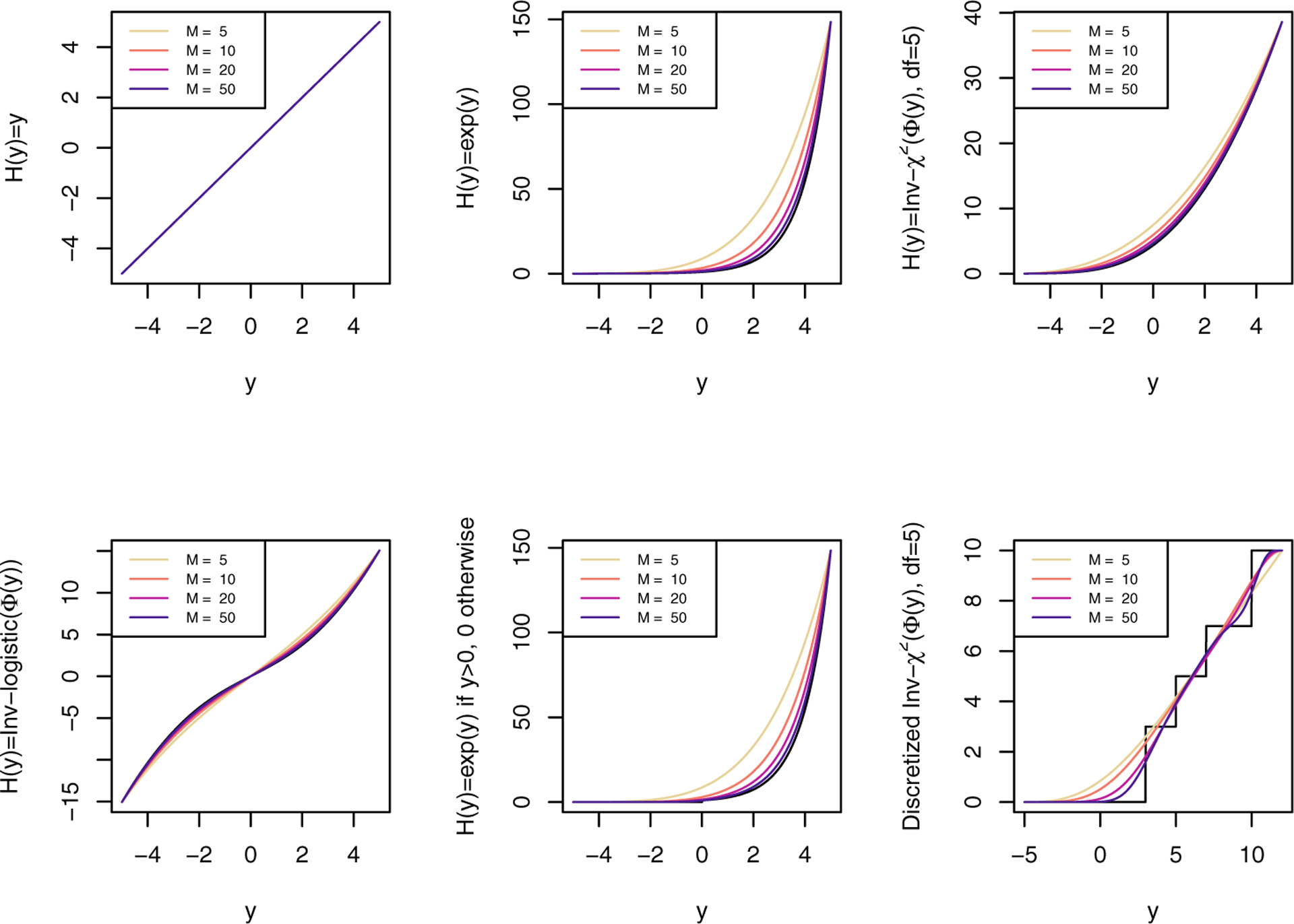
Transformation functions used in simulation and corresponding Bernstein polynomials approximation with order M

Note that the CDF in orm() is in the form G₁[1 − F (y|X)] = α_orm + β_ormX, which can be transformed to (2) if G(t) = −G₁(1 − t), α = −α_orm and β = β_orm. For symmetric error distributions, we use the same link function in orm() as in the CPM and α = − α_orm. For nonsymmetric error distributions, its complementary version can be used.³

3.2 |. Evaluations

To evaluate the two methods, we estimated bias, mean squared error (MSE) and coverage of 95% confidence intervals for β, as well as conditional expectations, conditional quantiles, and conditional cumulative distribution functions. We also computed the out-of-sample log-likelihood based on the fitted model parameters for a separate data set of the same size sampled from the simulation distribution. For the purpose of comparing the out-of-sample log-likelihoods, the responses in MLT were categorized into short intervals $({\underset{\_}{y}}_i,{\overline{y}}_i]$ based on CPM categorization, which were the distinct observed responses of the original data. The likelihood was then calculated as $L(H)={\prod }_i\left[F_{ϵ}\left(H\left({\overline{y}}_i\right)\right)-F_{ϵ}\left(H\left({\underset{\_}{y}}_i\right)\right)\right]$.

Under correct link function specification, for ϵ ~ N(0, 1), the probit link function was used and when ϵ followed a logistic distribution, the logit link function was used. We used the cloglog link function if ϵ followed a Gompertz distribution.

Ordinary linear regression was also evaluated and compared with the two methods for simple transformations H(y) = y and H(y) = exp(y). All simulations and analyses were performed in R version 3.4.4;¹⁶ complete code is available at http://biostat.mc.vanderbilt.edu/ArchivedAnalyses and an abbreviated version is available at https://github.com/harrelfe/rscripts/blob/master/sim-continuous-ordinal.r.

4 |. SIMULATION RESULTS

In general, CPMs and MLTs were quite comparable when models are correctly specified (i.e., correct link function and linear terms). Bias was close to 0, MSE was low, and the coverage probability of 0.95 confidence intervals tended to be 0.95 with increasing sample sizes. CPMs tended to have a slightly smaller bias for β than MLTs as the sample size increased. In terms of the conditional mean, CPMs generally had a smaller bias than MLTs, especially in large sample sizes, but MSEs were very close. Neither one had obvious advantages in estimating conditional quantiles. Both methods performed better estimating conditional medians than more extreme quantiles. CPMs generally had better performance in estimating conditional CDFs with a smaller bias, particularly in large sample sizes. MLTs tended to have slightly narrower confidence intervals. With continuous Y , the out-of-sample log-likelihood was larger in MLTs probably because it directly maximizes the likelihood whereas CPMs maximize an approximated multinomial likelihood. Details for specific simulation scenarios are provided below and in Supplementary Material.

4.1 |. The primary setting and its modifications

Simulation results under the primary setting, with the order of Bernstein basis varying from M = 5 to M = 10, are shown in Figure 2 and reported in Table S.1 (in Supplementary Material). For β estimation, CPMs and MLTs performed similarly, resulting in minimal bias and 95% coverage that improved with increasing sample sizes. CPMs had slightly less bias and similar to lower coverage than MLT with M = 10 when estimating conditional expectations. For estimating conditional CDFs and medians, MLTs with M = 5 generally underperformed MLTs of M = 10 and CPMs. Coverage of MLT with M = 10 was slightly better than that of CPMs for conditional CDFs and slightly worse for conditional medians. At large samples, estimates of conditional medians were less biased for CPMs than MLT with M = 10, but more biased at small sample sizes. For most of the remaining simulations, CPMs were only compared with MLTs with M = 10.

FIGURE 2.

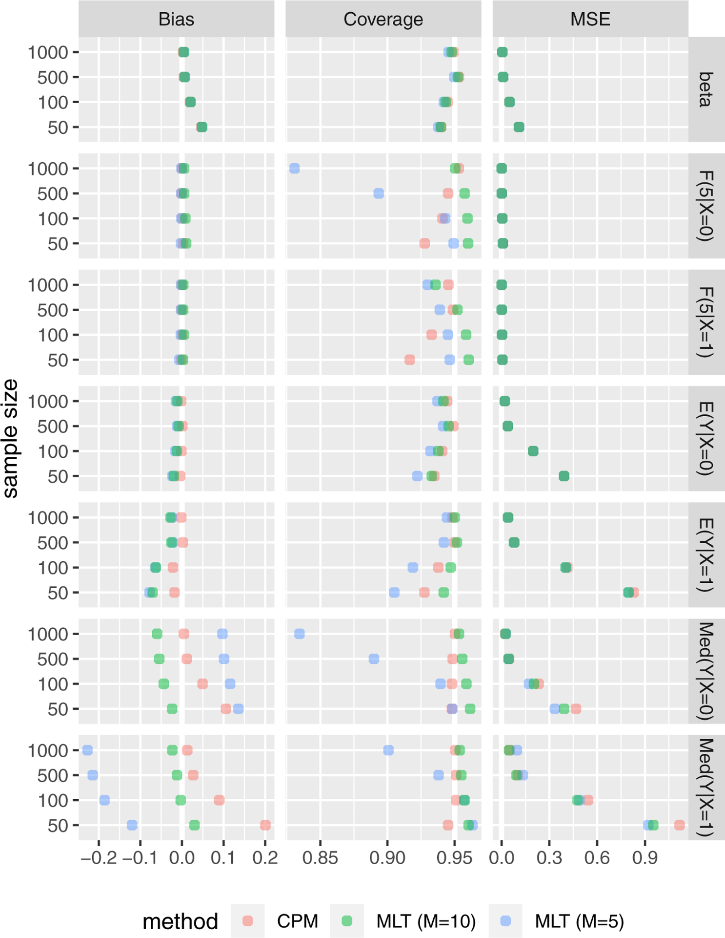
Simulation results under the primary setting

For simple transformations H(y) = y and H(y) = exp(y), ordinary linear regression after the correct transformation (i.e., no transformation and log-transformation, respectively) had, not surprisingly, the best performance in estimating β with much smaller bias, particularly at small sample sizes. The other two methods had similar respectable performance with coverage near 95% at all sample sizes and MSE 10% to 30% larger than the correctly specified linear regression, with MSE getting closer with larger sample sizes. The results of β estimation for transformation H(y) = y are in Table 1. With moderate and large sample sizes, the results of estimated conditional expectation were very similar. More detailed results are shown in Supplementary Material Figure S.1, Figure S.2, Figure S.3, Table S.2, Table S.3, and Table S.4.

TABLE 1.

Simulation results for β estimation of transformation H(y) = y

Sample Size	Method	Bias	MSE	Coverage (%)
n=50	CPM	0.0465	0.1077	0.9400
	MLT	0.0457	0.1068	0.9412
	Linear Regression	0.0003	0.0824	0.9399
n=100	CPM	0.0192	0.0491	0.9448
	MLT	0.0183	0.0487	0.9456
	Linear Regression	−0.0039	0.0403	0.9463
n=500	CPM	0.0045	0.0090	0.9532
	MLT	0.0043	0.0090	0.9537
	Linear Regression	0.0002	0.0080	0.9526
n=1000	CPM	0.0024	0.0046	0.9492
	MLT	0.0022	0.0046	0.9498
	Linear Regression	0.0001	0.0040	0.9518

When including a covariate Z, the results are shown in Figure 3. If Z was independent of X, MLTs had a slightly smaller bias in β and the differences between the two methods decreased as the sample size got larger. MSEs and confidence interval coverage rates were similar. However, if Z was dependent on X, the CPM had slightly better performance in estimating β than the MLT. In both scenarios, the MLT had a larger out-of-sample log-likelihood. When including multiple covariates, some of them being independent of X while others being dependent on X, CPMs generally outperformed MLTs although only by a small amount. (See detailed results in Table S.5, Table S.6, Table S.7, and Figure S.4 in Supplementary Material.)

FIGURE 3.

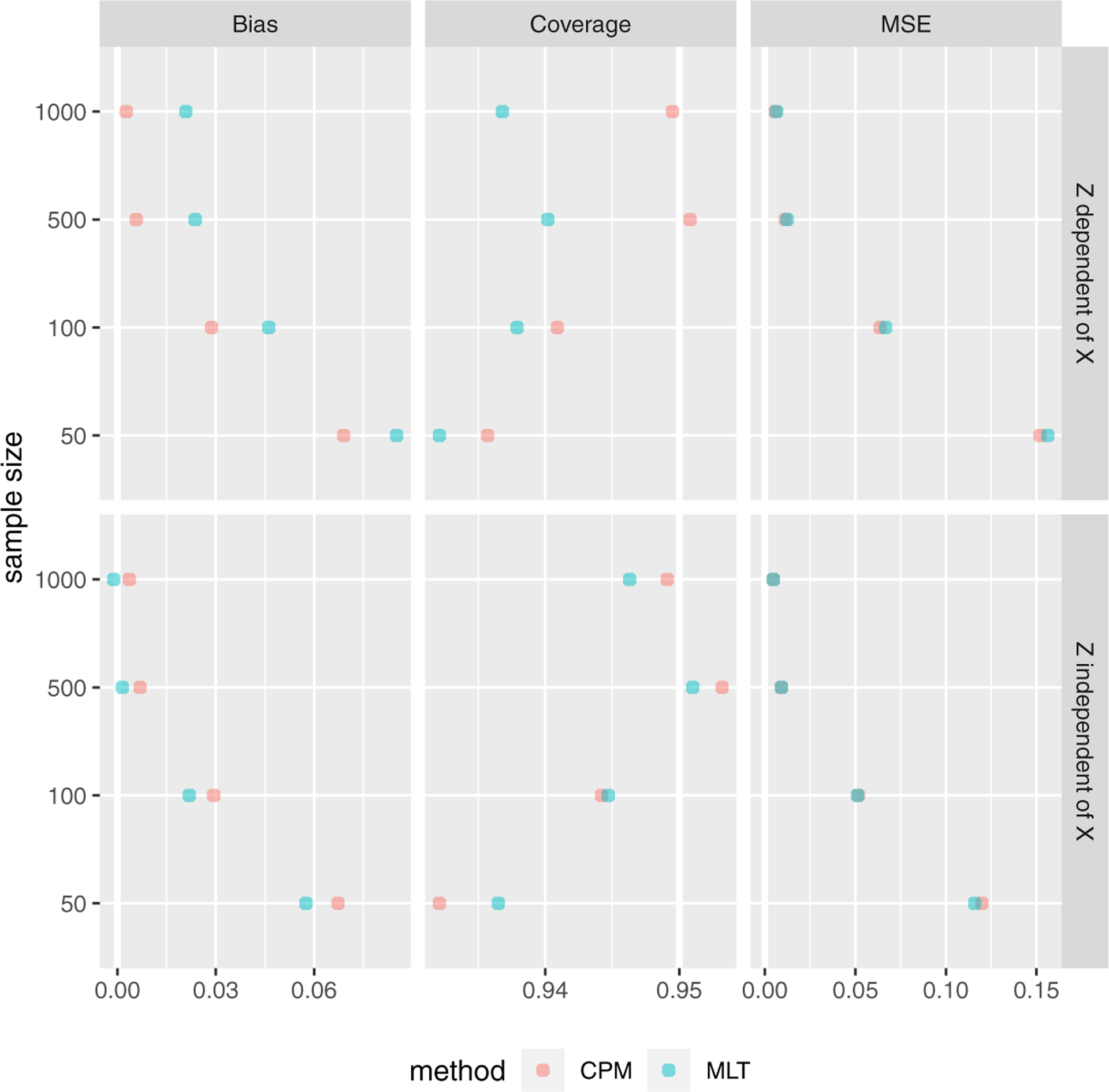
Simulation results when including covariate Z, which is dependent and independent of X

CPMs performed slightly better than MLTs when using the correct link function for $ϵ~\mathit{\text{Logistic}}\left(0,\frac{3}{{\pi }^2}\right)$ (See Table S.7 and Figure S.5 in Supplementary Material). Results were similar using correct link function for ϵ ~ Gompertz (See Table S.9 and Figure S.6 in Supplementary Material). Results were similar when using different distributions for X (see Supplementary Material Table S.10, Table S.11, Table S.12, Figure S.7, Figure S.8, and Figure S.9). When changing the value of β, the results were similar (see Supplementary Material Table S.13, Table S.14, Figure S.10 and Figure S.11).

4.2 |. Link function misspecification

Under minor or moderate link function misspecification, the bias of the estimated β was slightly smaller in CPMs. Results were similar in other evaluation criteria (See Table S.15 and Figure S.12 in Supplementary Material). With severe link function misspecification, MLTs tended to have slightly better performance in estimating β (See Table S.16, Table S.17, Figure S.13, and Figure S.14 in Supplementary Material). MLTs always had larger out-of-sample log-likelihood under model misspecification.

4.3 |. Mixture of discrete and continuous responses

For the mixture of discrete and continuous responses corresponding to the setting where values below zero were set to zero, we compared CPMs and two MLT models, one treating the responses as ordinary continuous responses and the second properly treating the zero values as left censored responses. For β estimation, the results are shown in Figure 4. For small sample sizes, the uncensored MLT had the smallest bias while the censored MLT and CPM had better confidence interval coverage rates. However, the uncensored MLT performed the worst when the sample size became large. CPM had the smallest bias in large sample sizes and it also had the largest out-of-sample log-likelihood in all sample sizes. See Table S.18 in Supplementary Material for more detailed results.

FIGURE 4.

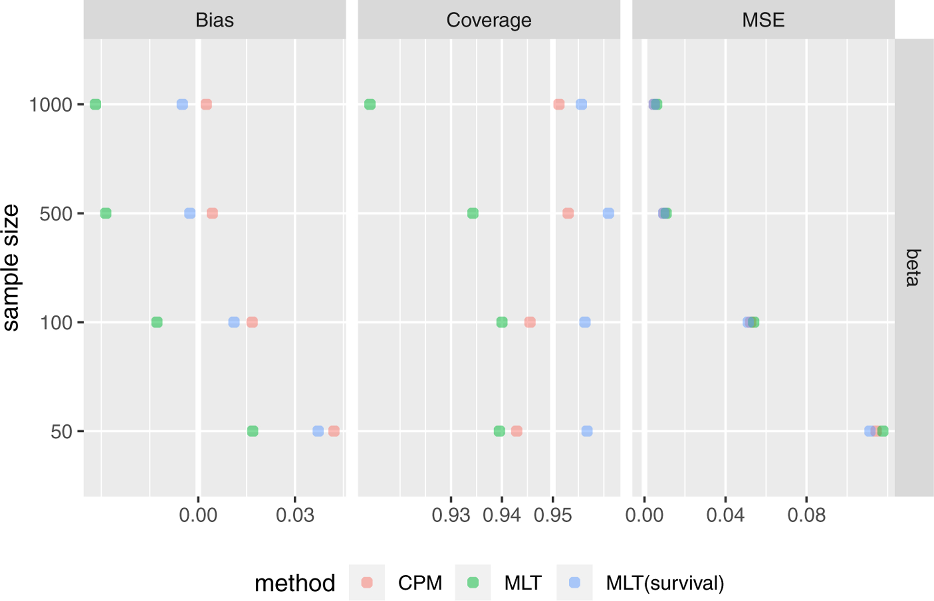
Simulation results for mixture of discrete and continuous responses comparing CPM and MLT treating response as ordinary continuous responses and censoring responses.

4.4 |. Discretization of continuous response

If continuous responses are discretized into categories, the MLT can handle them as ordered factors (i.e., resulting in identical estimation to CPMs) or as continuous responses. Simulation results are in Figure 5. CPMs, in general, performed better than MLTs (Bernstein polynomials with β = 5) treating the discrete data as continuous. Such advantages were more obvious as the sample size increased. MLTs outperformed CPMs for estimated β in sample sizes when the number of categories was small; while CPMs always had better confidence interval coverage rates for β. CPMs also had larger out-of-sample log-likelihood for all cases.

FIGURE 5.

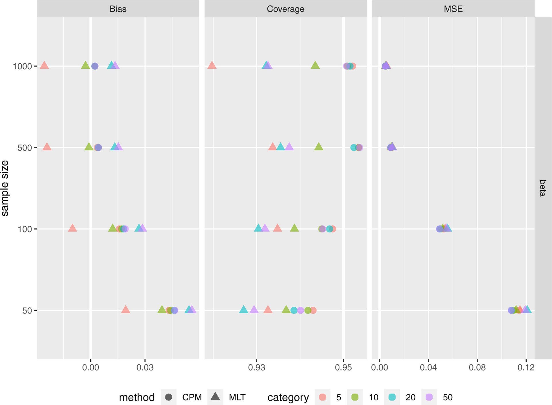
Simulation results for discretized continuous responses into 5, 10, 20 and 50 categories.

4.5 |. Computation time

The average computing time for the primary setting based on 100 replications is shown in Table 2. In general, both methods are quite fast for moderate sample sizes. On average, CPMs ran much faster in small sample sizes while MLTs were faster in large sample sizes. MLTs with M = 10 took longer to run than MLTs with M = 5. This simulation and all other simulations were performed on a 64 bit Linux server equipped with 2 Intel Xeon X5647 processors running at 2.93GHz, 96Gb of memory.

TABLE 2.

Average computation time (in seconds) for CPM, MLT(M = 5), and MLT(M = 10) for the primary simulation setting using different sample sizes and based on 100 replications

Sample Size	CPM	MLT(M = 5)	MLT(M = 10)
50	0.0349	0.1326	0.1729
100	0.0261	0.1360	0.1844
500	0.2909	0.2318	0.3121
1000	0.8703	0.3995	0.4416
10000	63.7773	2.8190	4.0533

5 |. APPLICATION EXAMPLES

To further compare the two models, we applied them to a biomarker study among people living with HIV (PLWH). The risks of diabetes and cardiovascular disease are higher for PLWH than the general population. There is interest in assessing the association between body mass index (BMI) and biomarkers of inflammation and metabolism among PLWH. We used data from 216 HIV-positive adults on antiretroviral therapy (ART) with no history of diabetes or myocardial infarction and with a viral load less than or equal to 400 copies/mL from the Vanderbilt Lipoatrophy and Neuropathy Cohort (LiNC; n=147)¹⁷ and the Adiposity and Immune Activation Cohort (AIAC; n=69).¹⁸ We estimated the association between BMI and five inflammation biomarkers: Interleuken 6 (IL-6), high sensitivity C-reactive protein (hsCRP), Interleuken 1 β (IL-1-β), soluble CD14 (sCD14) and leptin. The study over-sampled overweight patients; the median BMI was 29.3 kg/m²; the range was 17.8 to 57.4. The analysis adjusted for age, sex, race, study location, CD4 cell count, and smoking status. Probit link functions were used for all biomarkers.

Figure 6 shows the distribution of IL-6, which is right skewed and has a lower detection limit; those below the detection limit (3%) were recorded as having a value of 0. The estimated transformation functions are shown in Figure 6 and are similar for the CPM and MLT analyses. Because it is parametrically estimated by basis functions, the transformation function is a smooth curve for MLT. The transformation function for CPM is a step function. The estimated conditional mean and median as a function of BMI are also very similar for the two models. The estimated PI for IL-6 for a 10 kg/m² difference in BMI is 0.64 (95% CI 0.58–0.69) for both CPM and MLT analyses, further demonstrating the similarity between models. This suggests that for a 10 kg/m² difference in BMI, the subject with the higher BMI will have a 0.64 probability of having a higher IL-6.

FIGURE 6.

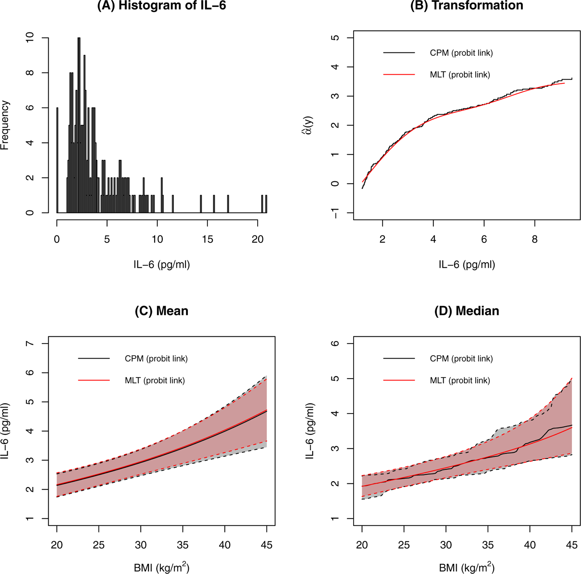
Results for IL-6. A: The distribution of IL-6. B: The estimated transformation functions. C: The estimated conditional means and their confidence intervals. Other covariates are at their most frequent level or median level. D: The estimated conditional medians and their confidence intervals. Other covariates are at their most frequent level or median level.

As shown in Figure 7, the distribution of hsCRP is extremely right-skewed. The estimated transformation is similar between the CPM and MLT analyses, but it is not as close as it was in the analyses with IL-6 as the outcome. Hence, the conditional expectation and the conditional median as a function of BMI are comparable, but slightly different, under the two transformation models. The probability indices for a 10 kg/m² increase in BMI are 0.59 (95% CI 0.54–0.65) and 0.60 (95% CI 0.55–0.65) for CPM and MLT, respectively. Interestingly, if one initially log-transforms hsCRP, fits MLT, and then transforms back to the original scale, then the MLT estimates are much more similar to those of the CPM; Figure 8 shows the conditional expectation. Notice that CPM is invariant to any pre-transformation transformation; i.e., estimates of β, expectations, quantiles, and probability indices are identical whether or not one applies an initial transformation. This is an advantage of CPM over MLT.

FIGURE 7.

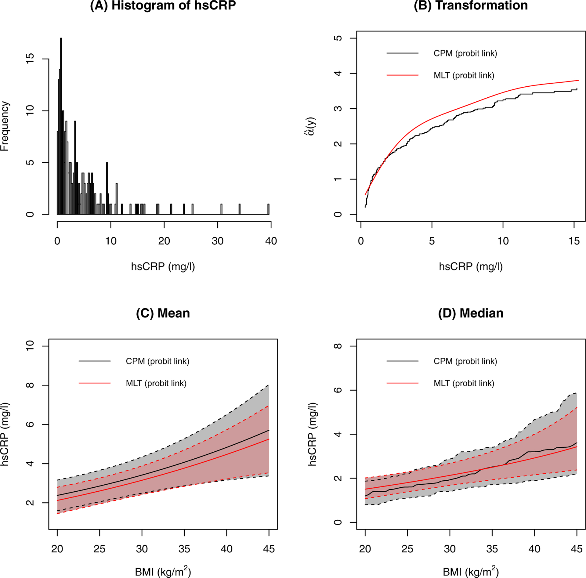
Results for hsCRP. A: The distribution of hsCRP. B: The estimated transformation functions. C: The estimated conditional means and their confidence intervals. Other covariates are at their most frequent level or median level. D: The estimated conditional medians and their confidence intervals. Other covariates are at their most frequent level or median level.

FIGURE 8.

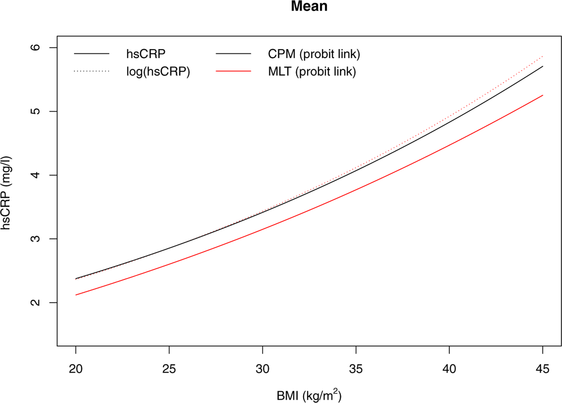
The comparison of the estimated conditional mean on the original scale and the transformed log scale

The distribution of IL-1-β is shown in Figure 9. It is right skewed and a large portion (39%) are below the assay detection limit and assigned the value 0. We applied CPM and MLT with left censoring to the data. The estimated transformation functions of the two models are somewhat similar. There is a flat line in the transformation function for CPM, which corresponds to the gap around 1 pg/ml in the histogram; CPM is flexible enough to capture this. The estimated conditional expectations are similar between the two models, with MLT generating a narrower confidence interval. The results for the conditional median are also similar for the two models. The PIs for 10 kg/m² difference in BMI is 0.50 (95% CI 0.44–0.56 for CPM and 0.44–0.55 for MLT) for both CPM and MLT, suggesting there is little association between BMI and IL-1-β.

FIGURE 9.

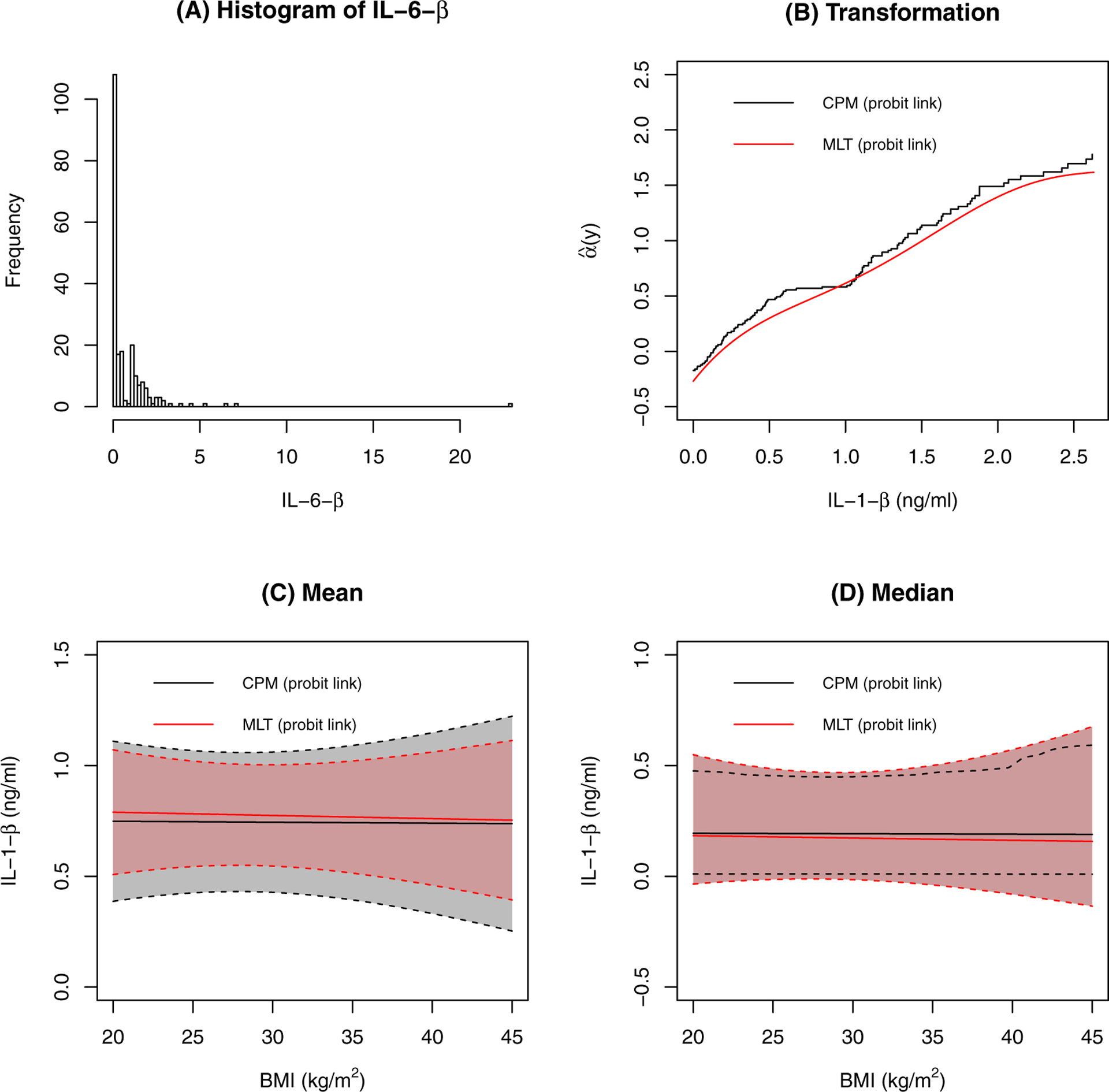
Results for IL-1-β. A: The distribution of IL-1-β. B: The estimated transformation functions. C: The estimated conditional means and their confidence intervals. Other covariates are at their most frequent level or median level. D: The estimated conditional medians and their confidence intervals. Other covariates are at their most frequent level or median level.

We also fit CPM and MLT models to assess the association between BMI and the biomarkers leptin and sCD14. Leptin was positively associated with BMI and sCD14 was negatively associated. In both cases, results from the CPM and MLT models were almost identical (similar to the IL-6 results); details are in Figure S.16 and Figure S.17 in Supplementary Material.

6 |. DISCUSSION

In this paper, we have reviewed two novel transformation models, CPMs and MLTs, and we have compared them under a variety of simulation settings. The paper also serves as a validation of the two software implementations in orm() and mlt(). Both methods directly model the conditional CDF from which other characteristics of the distribution can be derived easily. Both models are linear transformation models, in that they assume that after some transformation, the association between response and predictors can be characterized linearly with errors following a known distribution. The main difference between the two methods lies in the estimation of the transformation. CPMs are semiparametric transformation models; each distinct observed response is treated as a category and an ordinal regression model is fit which essentially models the transformation (or equivalently the intercept when written as a cumulative probability model) with a step function. With MLTs, the transformation is parametrically modeled using flexible basis functions. MLT also allows for easy set-up of more complex models featuring covariate-dependent effects using the low-dimensional parameterization of ϑ.^13,19

We ran extensive simulations to compare the two methods under different settings. The two methods had similar results in most cases and both methods handled complex transformations quite well. We had expected to see more gains in efficiency using MLT and more benefits in terms of robustness using CPMs; if this was the case, only minor differences were seen. MLTs were slightly more efficient. With larger sample sizes, the bias for MLTs occasionally slightly increased; this is presumably because MLTs are slightly misspecified with small orders (e.g. M = 10) and we kept the order constant irrespective of the sample size in our simulations. We ran another simulation using M = 15 with sample size of 1000 under the primary setting. The bias of conditional medians are −0.018 for X = 0 and −0.017 for X = 1, which are much smaller than the bias using M = 10. As illustrated with the biomarker data, CPMs are invariant to any monotonic transformation of the outcome, which can be considered an advantage. The CPM and MLT approaches handle censoring differently, with CPMs assigning values below a detection limit the lowest rank value, whereas MLTs assume that they follow a distribution informed by data above the detection limit. Resulting conditional expectations, therefore, are slightly different with MLTs treating censored values as something less than the detection limit whereas CPMs compute the expectation as the value after transforming the data back to the original scale (i.e., expectations will use the numeric value assigned to values below the detection limit). For computation time, MLT is significantly faster for large sample sizes with large numbers of distinct response values.

It should be emphasized that CPMs are semiparametric linear transformation models (SLTMs). SLTMs have been advocated for use with time-to-event outcomes and its parametric counterpart mlt() was employed to estimate Cox models with time-varying effects in Hothorn.²⁰ Some attempts have been made to use these models with continuous data,^6,7 but computation has been a limiting factor. By recognizing that ordinal “cumulative link models” are a special case of SLTMs and that algorithms applying ordinal models can be sped up using a few simple tricks implemented in the function orm of the R package rms, SLTMs can now be efficiently estimated as CPMs. It should be noted that most measurements in biomedical research are discrete to within the resolution of the measurement method. Results from semiparametric models treating the responses as discrete can in a sense be considered more accurate than continuous methods that approximate discrete responses using a smooth probability density function.

Although not the focus of this manuscript, diagnostics and goodness-of-fit can be assessed for both methods using probability-scale residuals and/or the probability integral transformation.^21,22,23 Since CPMs and MLTs both model the CDF, under proper specification with continuous responses, probability-scale residuals will be approximately uniformly distributed. Probability-scale residuals can also be used in residual-by-predictor plots and partial regression plots to investigate whether covariates are correctly included in the CPM or MLT models. Link functions can be selected based on an approach by Genter and Farewell.²⁴ Details and examples are in Liu et al.³

Future studies might consider even more flexible versions of transformation models. For example, it may be worthwhile to develop CPMs that permit different relationships and different distributions for different covariate levels. Extensions of both approaches to handle correlated or longitudinal data, using a similar approach to Manuguerra and Heller,²⁵ would also be beneficial.

AUTHOR BIOGRAPHY

Yuqi Tian. Yuqi Tian is a graduate student in the Department of Biostatistics at Vanderbilt University.

Torsten Hothorn. Torsten Hothorn is Professor for Computational Biostatistics at Universität Zürich.

Chun Li. Chun Li is Associate Professor of Biostatistics at Case Western Reserve University.

Frank Harrell, Jr. Frank Harrell, Jr. is Professor of Biostatistics at Vanderbilt University.

Bryan Shepherd Bryan Shepherd is Professor of Biostatistics at Vanderbilt University.

References

- 1.Box GE, Cox DR. An analysis of transformations. J R Stat Soc Series B. 1964;26(2):211–243. [Google Scholar]
- 2.Tukey JW. On the comparative anatomy of transformations. Ann Math Stat. 1957;28(3):602–632. [Google Scholar]
- 3.Liu Q, Shepherd BE, Li C, Harrell FE Jr. Modeling continuous response variables using ordinal regression. Stat Med. 2017;36(27):4316–4335. [DOI] [PMC free article] [PubMed] [Google Scholar]
- 4.Hothorn T, Möst L, Bühlmann P. Most likely transformations. Scand Stat Theory Appl. 2018;45(1):110–134. [Google Scholar]
- 5.Zeng D, Lin D. Maximum likelihood estimation in semiparametric regression models with censored data. J R Stat Soc Series B. 2007;69(4):507–564. [PMC free article] [PubMed] [Google Scholar]
- 6.De Neve J, Thas O, Gerds TA. Semiparametric linear transformation models: eėct measures, estimators, and applications. Stat Med. 2019;38(8):1484–1501. [DOI] [PubMed] [Google Scholar]
- 7.Zeng D, Lin D. Efficient estimation of semiparametric transformation models for counting processes. Biometrika. 2006;93(3):627–640. [Google Scholar]
- 8.Walker SH, Duncan DB. Estimation of the probability of an event as a function of several independent variables. Biometrika. 1967;54(1–2):167–179. [PubMed] [Google Scholar]
- 9.McCullagh P Regression models for ordinal data. J R Stat Soc Series B. 1980;42(2):109–127. [Google Scholar]
- 10.Harrell FE Jr. Regression Modeling Strategies: With Applications to Linear Models, Logistic and Ordinal Regression, and Survival Analysis. 2nd ed. New York: Springer; 2015. [Google Scholar]
- 11.Harrell FE Jr. rms: Regression modeling strategies. https://CRAN.R-project.org/package=rms. R package version 5.1–3.1; 2019. [Google Scholar]
- 12.Acion L, Peterson JJ, Temple S, Arndt S. Probabilistic index: an intuitive non-parametric approach to measuring the size of treatment effects. Stat Med. 2006;25(4):591–602. [DOI] [PubMed] [Google Scholar]
- 13.Hothorn T, Zeileis A. Transformation forests. arXiv preprint arXiv:1701.02110 2017. [Google Scholar]
- 14.Lindsey JK. Parametric Statistical Inference. Oxford: Oxford University Press; 1996. [Google Scholar]
- 15.Hothorn T mlt: Most Likely Transformations. https://CRAN.R-project.org/package=mlt. R package version 1.0–4; 2018. [Google Scholar]
- 16.R Core Team. R: A Language and Environment for Statistical Computing. Vienna, Austria: R Foundation for Statistical Computing; 2018. [Google Scholar]
- 17.Koethe JR, Bian A, Shintani AK, et al. Serum leptin level mediates the association of body composition and serum C-reactive protein in HIV-infected persons on antiretroviral therapy. AIDS Res Hum Retroviruses. 2012;28(6):552–557. [DOI] [PMC free article] [PubMed] [Google Scholar]
- 18.Koethe JR, Grome H, Jenkins CA, Kalams SA, Sterling TR. The metabolic and cardiovascular consequences of obesity in persons with HIV on long-term antiretroviral therapy. AIDS. 2016;30(1):83. [DOI] [PMC free article] [PubMed] [Google Scholar]
- 19.Hothorn T Transformation boosting machines. Stat Comput. 2019:1–12. [Google Scholar]
- 20.Hothorn T Most Likely Transformations: The mlt Package. J Stat Softw. Accepted 2018-03-05 https://cran.r-project.org/web/packages/mlt.docreg/vignettes/mlt.pdf. [Google Scholar]
- 21.Cox DR, Snell EJ. A general definition of residuals. J R Stat Soc Series B. 1968;30(2):248–265. [Google Scholar]
- 22.Li C, Shepherd BE. A new residual for ordinal outcomes. Biometrika. 2012;99(2):473–480. [DOI] [PMC free article] [PubMed] [Google Scholar]
- 23.Shepherd BE, Li C, Liu Q. Probability-scale residuals for continuous, discrete, and censored data. Can J Stat. 2016;44(4):463–479. [DOI] [PMC free article] [PubMed] [Google Scholar]
- 24.Genter FC, Farewell VT. Goodness-of-link testing in ordinal regression models. Can J Stat. 1985;13(1):37–44. [Google Scholar]
- 25.Manuguerra M, Heller GZ. Ordinal regression models for continuous scales. Inter J Biostat. 2010;6(1):14. [DOI] [PubMed] [Google Scholar]
Associated Data
This section collects any data citations, data availability statements, or supplementary materials included in this article.