CRediT Author Statement Principle ERP reduction and analysis: Estimating and using principle ERP waveforms underlying ERPs across tasks, subjects and electrodes

Abstract

Event-related potentials (ERP) waveforms are the summation of many overlapping signals. Changes in the peak or mean amplitude of a waveform over a given time period, therefore, cannot reliably be attributed to a particular ERP component of ex ante interest, as is the standard approach to ERP analysis. Though this problem is widely recognized, it is not well addressed in practice. Our approach begins by presuming that any observed ERP waveform — at any electrode, for any trial type, and for any participant — is approximately a weighted combination of signals from an underlying set of what we refer to as principle ERPs, or pERPs. We propose an accessible approach to analyzing complete ERP waveforms in terms of their underlying pERPs. First, we propose the principle ERP reduction (pERP-RED) algorithm for investigators to estimate a suitable set of pERPs from their data, which may span multiple tasks. Next, we provide tools and illustrations of pERP-space analysis, whereby observed ERPs are decomposed into the amplitudes of the contributing pERPs, which can be contrasted across conditions or groups to reveal which pERPs differ (substantively and/or significantly) between conditions/groups. Differences on all pERPs can be reported together rather than selectively, providing complete information on all components in the waveform, thereby avoiding selective reporting or user discretion regarding the choice of which components or windows to use. The scalp distribution of each pERP can also be plotted for any group/condition. We demonstrate this suite of tools through simulations and on real data collected from multiple experiments on participants diagnosed with Autism Spectrum Disorder and Attention Deficit Hyperactivity Disorder. Software for conducting these analyses is provided in the pERPred package for R.

1. Introduction

Electroencephalography (EEG) captures changes in voltage measured at the scalp, reflecting the firing of many similarly oriented neurons (Luck and Kappenman, 2011). When EEG recordings are time-locked to an event of interest, such as the onset of a trial or a participant’s response, event-related potential (ERP) waveforms are obtained. Through experimental designs utilizing contrasting task conditions, task-related changes to the ERP waveform are scrutinized to identify the “ERP components” that are thought to reflect particular brain processes. Subsequent studies – both in research and clinical settings – then seek to evoke and measure these ERP components in an effort to index the cognitive processes thought to generate them.

The goal of most ERP analyses, as described in the foundational text of Luck (2014), is “to provide an accurate measurement of the size and timing of the underlying ERP component with minimal distortion from noise and from other spatially and temporally overlapping components” (p285). Despite a number of approaches that seek to reveal underlying components of ERP waveforms as we do here, the standard approach for measuring ERP components is to take the average or peak amplitude over an investigator-selected time window, when the target ERP is expected to peak. This fails to remove the distortions from overlapping components, and the equating of components with peaks is deeply problematic.

Concretely, when an ERP component is defined and named, the functional process it reflects may be implied by virtue of the task and the contrast used to isolate it. However, in any subsequent study with different tasks and different participants, it can be problematic to attribute a peak that is observed at a similar time — or the potentiation/attenuation in it — to the same component, with the same functional meaning that was described in the previous studies. This is because a range of ongoing components may be differentially triggered by the different task conditions or participants. The overlapping activity of these unknown components can make the amplitude in a targeted interval higher or lower, and can push observed peaks/valleys in the waveform to occur either earlier or later in time. Moreover, even components typically associated with large peaks (such as the visual N1) may produce no observable peak as a result of such overlap.

These serious consequences of the overlapping nature of ERP components are widely recognized, including in the standard texts of Luck (2014) and Luck and Kappenman (2011). A less recognized problem with the common practice of taking an average or peak amplitude over a time window relates to the entire analytical tradition of targeting and reporting results for just one or several “components” from an ERP study. Such a selective approach to analyzing ERP experiments is understandable under the standard approach, where a reliance on selected intervals complicates efforts to characterize an entire waveform or to measure the magnitude of each component in a contributing set of waveforms, as we propose here. However focusing on so few features of the waveform limits what we can rigorously learn from our experiments, and slows the discovery of differences in components that may be of research or clinical value, all while amplifying selective-reporting concerns due to user-selection of these intervals.

In order to provide an alternative to the standard practice of using windowed peak or mean amplitude to define and measure ERP components, multiple approaches have attempted to decompose trial-wise or grand-averaged ERP waveforms into underlying sources which span the entire epoch. These approaches combine Principal Components Analysis (PCA) and Independent Component Analysis (ICA) techniques. Earlier works, beginning with Makeig et al. (1995) used ICA to carry out subject-level decompositions of the signal. Such subject-level decompositions require additional steps, generally relying on clustering techniques, in order to connect components extracted from one subject with those of others. This post-estimation clustering requirement is avoided by “multi-subject” decomposition approaches for ERP. The multi-subject decomposition of Spencer et al. (2001), called spatiotemporal PCA, involves two PCA steps: a “spatial” one that reduces the electrode dimension through PCA on data concatenated across subjects, and a “temporal PCA” to reduce the dimension in the temporal domain. Other multi-subject approaches, recently reviewed by Huster and Raud (2018), combine both PCA and ICA approaches for noise reduction and source separation, respectively. Multi-level Group ICA (mlGICA) of Eichele et al. (2011) and temporal-concatenation group ICA (tcGICA) of Cong et al. (2013) both consider trial-wise ERP and conduct one or two PCA steps for dimension reduction at the electrode or subject levels, followed by a final ICA step for source separation.

To introduce our approach, we begin with the core assumption: the observed ERP for any subject in any task/experiment and condition/trial-type, and at any electrode, is approximated by a linear combination of underlying waveforms spanning the entire epoch, called principle ERPs (pERPs). We propose the pERP-reduction (pERP-RED) algorithm to estimate these pERPs. The pERP-RED algorithm, similar in spirit to other multi-subject approaches, begins with two PCA-based noise reduction steps. The first to construct “regions” similar to the “virtual electrodes” of Spencer et al. (2001), but separately for each subject; the second to reduce the subject-region-task specific ERP averages into a smaller set that explains most of the sample variation. This is followed by an ICA step for blind source separation. However, pERP-RED has important differences from prior proposals. First, we emphasize that pERP-RED is designed for reducing data not only across multiple subjects but also across multiple tasks. Though this is not explicitly prevented by other methods, it is the intended use-case only for pERP-RED. A wider range of tasks/experiments stimulates a wider range of neural processes, each with their own signatures that get mixed into the observed signal, which we seek to separate out and measure. The multi-task approach of pERP-RED takes advantage of this rich form of data and estimates a set of pERPs with greater generalizability. Another useful benefit of the multi-experiment setting, in this early validation stage, is that it allows a test of whether different tasks, trial types or conditions are built up from shared components in the expected ways. Second, the electrode dimension reduction PCA steps of spatial PCA, mlGICA and tcGICA, all performed on matrices concatenated over subjects or trials, assume no missingness on electrodes, identical trial orderings, identical scalp topographies, or identical projections of components onto electrodes across subjects. The electrode reduction PCA step of pERP-RED, by comparison, avoids these assumptions by running dimension reduction separately for each subject in the first step. Subject-region-task specific ERP averages are only combined at the second PCA noise reduction step, which does not assume any homogeneity over the subject-specific components concatenated from the first step.

However, more important than these algorithmic differences, our approach is unique in arguing for a new way to analyze one’s data using these pERPs, and the set of tools we develop and make available to do so. Despite existing algorithms for estimating underlying components, the standard practice of using windowed peak or mean amplitudes continues to dominate in most published ERP studies. We argue that much more can and should be done to analyze one’s ERP waveforms using these underlying components than has been the case in any prior work. Our primary objective is to provide researchers with a set of analytical tools for examining their ERP experiments in terms of these components, which we call “pERP-space analysis”. That is, rather than attempting to measure a single component’s magnitude, coefficients describing the contribution of all pERPs in any given ERP waveform can be estimated and reported. These estimated pERP coefficients are directly interpretable as the magnitude of each pERP’s contribution to the observed waveform, and are equipped with standard errors. This allows the practitioner to analyze and report both the presence/absence and the strength of each pERP in each condition, group or scalp region, and to make inferences on condition or group contrasts. Additionally, we provide tools to track across-subject heterogeneity of the magnitude of each pERP’s contribution (e.g. heterogeneity in the pERPs, for anxious vs. non-anxious youth). By characterizing entire ERP waveforms in terms of these contributions (and their heterogeneity) rather than one or several time windows, this approach greatly facilitates the discovery of unexpected differences that may prove to be useful in research or clinical application, while better limiting user discretion (e.g. the choice of interval) and selective reporting (of one component/interval rather than others).

We outline the proposed pERP-RED algorithm and pERP-space analysis steps in the next section. Properties of the proposed approach are demonstrated using simulations (Section 3) and two separate real data examples (Section 4), each employing multiple tasks to derive a common set of pERPs followed by pERP-space analyses. Finally, to increase accessibility we provide an R package, pERPred. Investigators may keep their current pre-processing procedures and workflows up to and including the step of generating ERP waveforms at the subject level. These can then be imported into our software, allowing pERPs to be estimated and all the pERP-space analyses to be visualized through a graphical interface employing simple drop-down menus. We also make results available for the applied examples here through a publicly available browser-based implementation of that interface to encourage exploration and familiarization with the proposed pERP-space analyses.

2. Methods

In what follows we provide a detailed description of both the pERP-RED algorithm used to derive pERPs from an original dataset possibly spanning many participants, groups, and tasks, and then a set of tools that comprise the pERP-space analysis that we foresee being of value to a wide audience of investigators for the practical use of pERPs in research.

2.1. The pERP-RED Algorithm

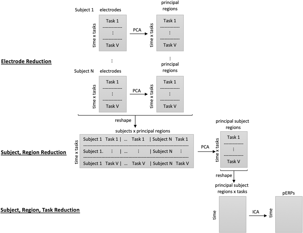
The pERP-RED algorithm is motivated by the goal of estimating an underlying set of component waveforms, herein referred to as pERPs, such that the ERPs formed by time-locked averages at any given electrode, participant, or trial type is approximately a weighted combination of these components. Our approach, depicted in Figure 1, involves (i) a series of data concentrating steps that turn a larger number of noisy waveform records (i.e. average ERPs for a given trial type, participant, electrode) into a smaller number of less noisy ones; and (ii) steps that generate maximally independent, “unmixed” components from these concentrated signals. Unlike some related approaches (such as spatiotemporal PCA, Spencer et al. 2001) we do not conceptualize steps nor results as either “temporal” or “spatial” in the data reduction; rather we estimate the pERPs thought to underlie all ERPs (across all subjects, electrodes, and tasks) first, after which it is possible to both see how these load onto a given waveform and to see how these loadings are spatially distributed.

Figure 1:

Illustration of the pERP-RED algorithm, described in text. First, at the within-subject level, correlation across electrodes is used to estimate a smaller number of “principal regions” for each subject, which we term “subject-region” scores. Next, these subject-region scores are combined together across subjects, then reduced to “principal subject-region” scores. These data are then reshaped to give separate columns for each principal subject-region score on each task/condition. The resulting waveforms are decomposed by ICA in order to arrive at the final pERPs.

To describe these in detail, we first set notation. Let i denote subjects, i = 1,...,N; υ tasks, υ = 1,...,V; e electrodes, e = 1,...,E_i; t the number of time points, t = 1,...,T; and p the number of pERPs, p = 1,...,P. Note that each subject not only have electrodes in slightly different locations on the scalp, but may also have different numbers of electrodes owing to dropped channels after data cleaning steps. By beginning with the reduction of electrodes to “regions” within subject, this is unproblematic. The steps of the pERP-RED algorithm are then:¹

1. Data initialization. Data are first split, by subject into a training set and test set. Normalize each of the resulting ERPs to have unit variance. Proceed to next steps using only the training set.

2. Electrode reduction. The first data concentration or reduction step transforms electrode-level data within each subject to “region” level data within subjects, thereby reducing the electrode dimension. This is done by applying PCA to each of the N subject-specific matrices of size (T × V ) × E_i, with data across electrodes in the columns and each tasks’ data concatenated in the rows. This produces N matrices of size (T × V) × R_i, where R_i is the number of principal regions that explains a pre-specified amount of variance. By default we set this threshold at 80%.

3. Subject-region reduction. The second data reduction step begins by reshaping the above data into a matrix of size $(T\times V)\times \left({\sum }_{i=1}^N{R}_i\right)$ with all of the principal regions as the columns and the task and time dimensions concatenated in the rows. Each task-region ERP record is normalized to unit variance. Then PCA is used to generate N_R principal subject-regions.

4. Source separation. The data are then reshaped into a matrix of size T × (V × N_R) with all task principal subject-regions as the columns and time as the rows. Fast ICA is then used to produce P principle ERPs, where P may be chosen by regressing the true signal (in the test set) onto the components and obtaining an R² value.

We make several remarks on these choices. First, in this paper, we use subject-level averages over trials of a given type as the “records” that first enter the algorithm above. This need not be the case: if for example one is interested in practice effects, then earlier trials and later trials may be averaged separately. Note that even having averaged trials together within participants, once the pERPs are estimated, it is still possible to go back and examine whether the amplitudes of pERPs vary from earlier trials to later trials (we further discuss the analysis of these amplitudes below). Hence one need not posit that “all the trials being averaged together are the same”, and variation in how pERPs contribute to different trials in the original, un-averaged data can still be studied. Statistically, the only requirement is that the data that enter the algorithm should include various weightings of the underlying components we aim to recover. Records need not (and certainly will not) be homogeneous in these components or mixtures of them. Put differently, any averaging that occurs prior to beginning the algorithm above should not “annihilate” or cancel out any components that would otherwise have been of interest.

Next, the purpose of splitting the data into a training and test set is to allow us to choose the appropriate dimensionality of the data in the final step, and to allow an unbiased evaluation of how well the principle ERPs explain the signal in a set of subjects not used to derive those principle ERPs. We use 2/3 for training and 1/3 for testing but this choice is left to the user. Once the training-test set split has been used to decide upon the number of components, the components are re-estimated using all of the data.

At each data reduction step, we normalize the records. Equivalently, the covariance matrix underlying the PCA steps is actually a correlation matrix. In the “electrode reduction” step, the aim is to go from a large number of electrodes that may have highly correlated signals to a smaller set, each of which provides uncorrelated information relative to the others. That is, if we imagine a set of electrodes that all have a correlation of nearly one or negative one with each other, we would choose to collapse these into a single signal. We call the resulting principal components “regions”, though they need not and likely will not reflect coherent spatial regions. The subsequent “subject-region reduction” is analogous: if there are groups of participants that have “region” (combined electrode) signals that are highly correlated, this information can be combined with little loss.

In the final step, we use ICA rather than PCA because the aim is to take the “concentrated” data from the two reduction steps, and estimate components that are believed to be maximally independent. It thus resembles a blind source separation problem for which ICA is well suited, much as it is widely applied in source localization algorithms. This does not imply that the resulting components are functionally independent or meaningful sources.

Several choices remain user-driven at present. The first regards the proportion of variance each of the PCA steps must explain during the data concentration steps. Keeping a larger number of components implies that more of the data will survive into the final estimates, but at the cost of keeping more noise as well. It can also become computationally costly. Our supposition in choosing to keep enough components to cover 80% of the variation is that this should be sufficient to recover almost all of the true signal of value, whereas going beyond this is apt to introduce mostly noise.

The ICA step, too, requires choosing the number of components to estimate, P. In principle, V × N_R independent components can be kept. However there is no reason to expect that there are exactly V × N_R meaningful signals to separate. The risk of estimating too many components is that over-decomposition may occur, splitting single meaningful components into separate estimated sources. Similarly, the risk of estimating too few components is that under-decomposition occurs, with separate sources remaining “mixed” together to alias as one (see e.g. Kairov et al. 2017). In our case, over-decomposition is less harmful, because we will later characterize a given ERP waveform according to the linear combination of pERPs that compose it. The estimated pERPs can thus still “work together” to explain the average ERP for a particular condition, group or person. Thus, over-decomposition will simply lead to a wider set of pERPs being implicated and discussed as contributing to a given waveform or contrast.

Subject to this, however, the smallest set of components that will suffice is preferable for purposes of analysis and interpretation. We choose the number of final components P according to how well this set can explain actual ERP data, in a test set not used to estimate the pERPs. Denote the estimated pERPs as Φ = [Φ₁, Φ₂,...,Φ_P]. Let j = 1,...,J be a counter running over each condition, subject, and electrode combination in the test set, with Y_j being the observed ERP record for the j^th condition/group/electrode. Without loss of generality, assume Y_j has been demeaned. Each of the J observed ERPs in the test set are then regressed individually on the matrix of the estimated pERPs, fitting the model

$$Y_j=\text{Φ}{\beta }_j+{ϵ}_j.$$

The variance in the test ERPs explained by the pERPs is then

$$R_{\text{test}}^2=1-\frac{{\Vert Y_j-\mathrm{\Phi }{\beta }_j\Vert }_{\mathcal{F}}^2}{{\Vert Y_j\Vert }_{\mathcal{F}}^2}$$

where $\Vert \cdot {\Vert }_{\mathcal{F}}^2$ denotes the Frobenius 2-norm, which corresponds effectively to a variance times N. We then choose the number of pERPs, P, such that raising P would result in relatively little additional gain in $R_{\mathit{\text{test}}}^2$. Once P is chosen, all the data (in the training and test sets) are used to re-estimate the pERPs that will be used in the pERP-space analysis. We demonstrate this below.

2.2. The pERP-Space Analysis

The above procedure describes our proposal for how pERPs can be obtained. We now turn to how the estimated pERPs can be used in a complete analytical approach that avoids the problems inherent in the practice of using windowed peak (or mean) amplitude. The central concept is that any observed ERP waveform (for some condition over some group or individual at some electrode) can be recast as a vector of coefficients describing the magnitude of each pERP’s contribution to that ERP.

Step 1: Individual scoring.

We start by using pERPs to extract data about a condition within an individual. Here condition refers to trial types within a single experiment, such as match and mismatch conditions within the audio paradigm of Section 4.1. For individual i and condition c, at electrode e, let the observed ERP be denoted by the vector Y_i,c,e. Henceforth we suppress the electrode index, e, for simplicity. Let Φ be the matrix whose columns contain the pERPs. We first regress Y_i,c on the pERPs to obtain coefficients,

$${\omega }_{i,c}=({\text{Φ}}^{\text{T}}\text{Φ}{)}^{-1}{\text{Φ}}^{\text{T}}{Y}_{i,c}.$$ (1)

The vector ω_i,c can thus be thought of as a vector of coefficients, amplitudes, loadings, or weights that encode the ERP Y_i,c in terms of the contributions of each pERP. As ω_i,c is a vector of size P by 1, with each element representing loadings onto each pERP, operations performed on such vectors below (such as subtraction or averaging) are performed element-wise. Note that this brings about a substantial dimension reduction: ERPs that contain 1000 data points are represented using only 10–15 dimensions in the empirical examples explored below while explaining 80–90% of the total variation.

Second, when investigators are interested in a between-condition contrast, we also extract that contrast at the individual level. That is, suppose we are interested in how condition c compares to condition c′, obtaining ω_i,c−c′ = ω_i,c − ω_i,c′. If done literally, this implies computing (Φ^TΦ)⁻¹Φ^TY_i,c − (Φ^TΦ)⁻¹Φ^TY_i,c′. However, note that this is numerically the same as (Φ^TΦ)⁻¹Φ^T(Y_i,c − Y_i,c′), which first differences the ERPs for condition c and c′ within subject i before regressing them on Φ. The benefit of doing this differencing within-subject is that later statistical tests that assume independence across subjects but not across conditions within subject will remain valid.

Finally, to reduce redundancy in what follows, we use the notation ω_i,c−c′ generically even where investigators may be interested only in comparing scores from condition c to a null value of zero, and not to another condition.

Step 2: Summary across individuals.

The values of ω_i,c−c′ can then be regarded as data representing individual i’s response on condition c compared to c′ (or on c alone if c′ is omitted). These are measurements that can be summarized by conventional statistics such as the mean and standard deviation, while the mean can then be characterized by its standard error. We construct these quantities next.

Over all individuals, the mean vector, $\overline{\omega }$_c−c′, of size P by 1, would be given simply by $\frac{1}{N}\sum _i{\omega }_{i,c-c^{\prime }}$. We further consider group-wise means written as

$$\overline{\omega }{(g)}_{c-c^{\prime }}=\frac{1}{N_g}\sum _{i\in G_g}{\omega }_{i,c-c^{\prime }}$$

for group g, where G_g denotes the set of indices, {i}, for subjects falling in group g and N_g denotes the size of the group.

To describe variability in the loadings across individuals in group g on condition c or on the contrast of c and c′, we construct the standard deviation within the group. For clarity we label this the across-person standard deviation (APSD) for group g,

$$APSD{(g)}_{c-c^{\prime }}=\sqrt{\sum _{i\in G_g}\frac{{\left({\omega }_{i,c-c^{\prime }}-\overline{\omega }{(g)}_{c-c^{\prime }}\right)}^2}{N_g-1}}.$$

Finally, to facilitate inferences about group-wise means or mean contrasts, we construct the standard errors that reflect the variation in those means,

$$SE{(g)}_{c-c^{\prime }}=\sqrt{\frac{\sum _{i\in G_g}\frac{{\left({\omega }_{i,c-c^{\prime }}-\overline{\omega }{(g)}_{c-c^{\prime }}\right)}^2}{N_g-1}}{N_g}}.$$

Step 3: Description and inference.

With these statistics, the investigator can perform a range of analyses. A first question is how much each pERP contributed to a given condition (c) or contrast (c − c′). This can be tested for any grouping g, by constructing

$$t{(g)}_{c-c^{\prime }}=\frac{\overline{\omega }{(g)}_{c-c^{\prime }}}{SE{(g)}_{c-c^{\prime }}}.$$

Note that the tests would be carried out element-wise on the P elements of t(g)_c−c′, corresponding to contributions from the P pERPs. If we are interested in knowing which pERP contributed with a detectably non-zero weight to a given condition c, this would be done for a single condition c (i.e., “setting c′ to zero”). If we would instead like to know if the difference in contribution of any pERP to condition c versus c′ is distinguishable from 0, then this would employ both c and c′. Note that the proposed approach can be used to quickly “screen” ERPs to determine which pERPs are contributing detectably non-zero amounts to a given condition or contrast. Our suggested reporting style, as illustrated below, would automatically provide such t-statistics (and associated p-values) for all pERPs in a table. This avoids selective reporting and aids in discovering unexpected differences, while producing a fixed number of tests.

Second, we may be interested not only in which pERP contributes to a given condition or contrast for individuals in group g, but how this differs from what we see in group g′. We can similarly construct

$$t{\left(g,g^{\prime }\right)}_{c-c^{\prime }}=\frac{\overline{\omega }{(g)}_{c-c^{\prime }}-\overline{\omega }{\left(g^{\prime }\right)}_{c-c^{\prime }}}{\sqrt{SE{(g)}_{c-c^{\prime }}^2+SE{\left(g^{\prime }\right)}_{c-c^{\prime }}^2}}$$

to test against the null hypothesis that two groups/conditions have the same mean contributions from each pERP. Note that the intended usage here is for non-overlapping groups g and g′, which we treat as independent samples. Such contrast statistics can also be reported on all pERPs in table form for transparency. Again we illustrate this usage below, and such tables are automatically generated in the software provided.

Third, investigators may be interested not only in how pERP loadings on a condition or contrast vary between groups, but in whether certain groups have higher/lower variability than others. They can thus compare APSD(g)_c−c′ across groups. Fourth, recalling that ω quantities are available at each electrode e, topographic head maps can be shown as well for conditions/constrasts such as $\overline{\omega }$(g)_c−c′ or for between-group differences in conditions or contrasts, $\overline{\omega }$(g)_c−c′ − $\overline{\omega }$(g′)_c−c′. These can be shown either for these magnitude estimates themselves, or on the corresponding t-statistics to give a sense of statistical scale. We show examples in our applications below and provide this functionality in the software.

Other uses of pERPs

We note several other potential use cases that are less analagous to traditional ERP analysis of components but serve as additional uses for ω_i,c−c′ values once extracted. First, investigators may wish to compare ω_i,c−c′ to behavior or clinical measures for person i. Second, pERPs provide a means of ERP “cleaning”: one can reconstruct ERPs using only the derived pERPs. This leaves out components of the signal that have been deemed to be noise. Such a cleaning approach may be especially useful when visualizing individual or single-trial ERPs.

Third, the pERP analysis approach could in principle be used for participant rejection as well. Specifically, individuals for whom the pERPs collectively explain less of their signal must be very noisy, suggesting problems in data collection, or at least pointing to their divergence from the rest of the sample. Fourth and finally, the pERP-space analysis can also be used for outlier detection: individuals with very unusual values of ω_i,c−c′ could be examined.

3. Simulation

The proposed pERP-RED algorithm is studied extensively through simulations in which the sample size, correlation among electrodes and tasks, percent of variation used to retain PCA components and signal-to-noise-ratio are varied. In addition to assessing the efficacy of pERP-RED, the simulations also target providing readers guidance on the choice of tuning parameters and comparing pERP-RED to alternate algorithms. Depending on the amount of noise in the simulated data, the run time of pERP-RED ranges between 4 and 30 minutes (longer for more noise) at N = 50 when parallelized on a 2.4 GHz 6-Core Intel Xeon processor operating R 3.6.2 (R Core Team, 2019).

3.1. Simulation Design

The observed signal is assumed to be a linear combination of the pERPs. Let Y_i,v,e(t) denote the ERP signal observed for subject i at task v and electrode e. Note that we employ here the term “tasks” to refer to trial types generally, possibly defined across experiments, whereas the term “condition” refers to trial types within an experiment. The data generation model used in the simulation is:

$$Y_{i,v,e}(t)=\sum _{p=1}^P{k}_{p,v,e}{\varphi }_p^{\star }(t)+\sum _{p=1}^P{\xi }_{p,i,v,e}{\varphi }_p^{\star }(t)+\sum _{\mathcal{l}=1}^L{\alpha }_{\mathcal{l},i,v,e}{\psi }_{\mathcal{l}}(t)+{\zeta }_{i,v,e}(t),$$ (2)

Where ${\varphi }_p^{\star }(t)$, ψ_ℓ(t) and ζ_i,v,e(t) denote the “true” pERPs, Fourier basis functions and measurement error, respectively and k_p,v,e denotes the task- and electrode-specific weights, and ξ_p,i,v,e and α_ℓ,i,v,e denote the subject-, task- and electrode-specific weights of the respective bases decompositions. The total number of tasks, denoted V, the total number of true pERPs, denoted P, the total number of time points, denoted by T, the total number of Fourier bases, denoted by L, and the total number of electrodes per subject, denoted by E, are set to equal 9, 5, 500, 7, and 40, respectively.

The first term in (2) reflects that ERPs observed at each task and electrode are composed of a weighted average of the true pERPs, denoted by ${\varphi }_p^{\star }(t)$. To simulate a single ${\varphi }_p^{\star }(t)$, we draw a function from a reproducing kernel Hilbert space of smooth, relatively low frequency functions. The functions in this space are simply the superposition of rescaled Gaussian kernels “centered” around different time-points. Specifically, ${\varphi }_p^{\star }(t)$ is the summation of 20 rescaled kernel functions, ${\varphi }_p^{\star }(t)=\sum _{m=1}^{20}{a}_m\mathit{exp}(-{(t-t_m)}^2/h_p)$, where the center t_m of each kernel is chosen uniformly from [0, 1], and the kernel bandwidth h_p is set to 0.3(−0.125 + 0.375p). The coefficients a_m rescaling each kernel is drawn from a uniform (0, 1) distribution. These simulated signals are then rotated by ICA to form a maximally independent set of bases. The coefficients, k_p,v,e, are drawn independently from a normal distribution with mean zero and variance ${\sigma }_k^2=0.25$.

The second term in (2) represents subject-specific deviations from task- and electrode-specific signal. The subject-specific weights ξ_p,i,v,e are drawn from a matrix normal distribution (to create a dependence structure within tasks and across electrodes) with mean zero and covariance matrices Σ_p,v and Σ_p,e of dimension V * V and E * E (identically and independently drawn over subjects). The covariance matrices for the P = 5 total pERPs are created in the same way for the electrode and task dimensions, starting out with a matrix of 1 on the diagonal and the correlation ρ elsewhere. The value of ρ will be varied to assess the effects of tuning parameter choices outlined in Section 3.2. These covariance matrices are then multiplied by a factor of 0.1(P − p), for p = 1,...,5, respectively, so that each true ERP component is represented differently.

The third term in (2) represents a noise component that is structured in time. The Fourier bases contain ψ₀(t) = 1, and pairs of sine and cosine functions ψ_2r−1(t) = $\sqrt{2}$ sin(2πrt) and ψ_2r(t) = $\sqrt{2}$ cos(2πrt) for r = 1,..., (L − 1)/2, with L = 7. The coefficients α_ℓ,i,v,e are generated in the same way as ξ_c,i,v,e. Specifically, α_ℓ,i,v,e are drawn from a matrix normal distribution with mean zero and covariance matrices Σ_ℓ,v and Σ_ℓ,e which equal 1 on the diagonal and ρ on the off diagonal terms. The covariance matrices are multiplied by a factor of 0.05(ℓ + 1) for ℓ = 1,...,7.

The last term in (2) is the independent and identically distributed measurement error. The measurement error ζ_i,v,e(t) is generated (independently over i, υ, and e) from a normal distribution with mean zero and variance ${\sigma }_{\text{error}}^2$. The variance ratio of the signal $\sum _{p=1}^P{k}_{p,v,e}{\varphi }_p^{\star }(t)+\sum _{p=1}^P{\xi }_{p,i,v,e}{\varphi }_p^{\star }(t)$ to noise $\sum _{\mathcal{l}=1}^L{\alpha }_{\mathcal{l},i,v,e}{\psi }_{\mathcal{l}}(t)+{\zeta }_{i,v,e}(t$ is varied in different simulation set-ups to equal 0.6 and 1, referred to as the high and low noise cases, respectively.

3.2. Simulation Results

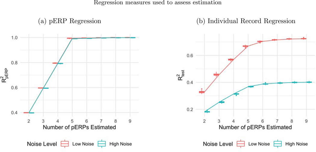
The estimation accuracy of pERP-RED is assessed using two measures: $R_{\text{test}}^2$ and $R_{\text{pERP}}^2$. The first measure $R_{\text{test}}^2$ is calculated in the last step of the pERP-RED algorithm as given in (2.1) to assess the estimation accuracy of the predicted records in the test set. The second measure, denoted by $R_{\text{pERP}}^2$, assesses the performance of pERP-RED in targeting the true pERPs, which can only be estimated in simulations. To obtain $R_{\text{pERP}}^2$, the matrix of true pERPs ${\mathrm{\Phi }}^{\star }=\left[{\varphi }_1^{\star },\dots ,{\varphi }_5^{\star }\right]$ is regressed on the estimated pERPs Φ = [ϕ₁,...,ϕ_P] to determine the degree to which linear combinations of the estimated pERPs can account for (any linear combination of) the true pERPs used in the simulation. That is: how accurately did we recover the true pERPs, up to rotations? $R_{\text{pERP}}^2$ is then given by the proportion of variance in the true pERPs explained by the estimated ones

$$R_{\text{pERP}}^2=1-\frac{{\Vert {\mathrm{\Phi }}^{\star }-{\widehat{\mathrm{\Phi }}}^{\star }\Vert }_{\mathcal{F}}^2}{{\Vert {\mathrm{\Phi }}^{\star }\Vert }_{\mathcal{F}}^2},$$

where ${\widehat{\mathrm{\Phi }}}^{\star }$ is the prediction of the true ERPs given by the estimated ones.²

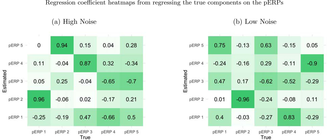
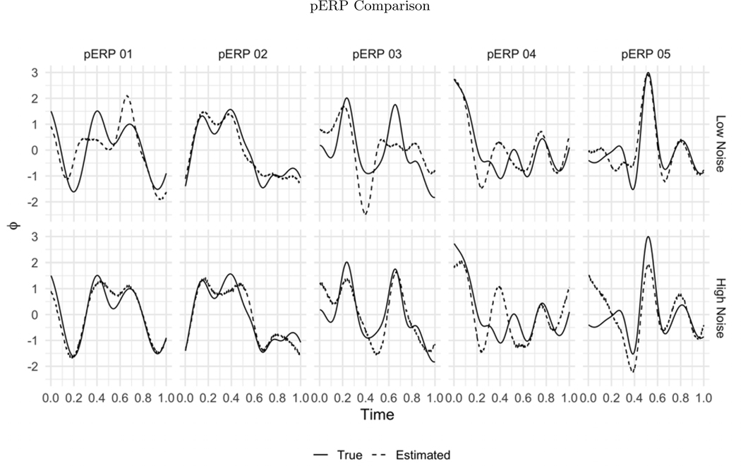
Before summarizing results from multiple simulation settings corresponding to varying sample sizes, correlations among electrodes and tasks and percent of variation used to retain PCA components, we present results from a single simulation set-up with N = 50, ρ = 0.5 (medium correlation induced among of tasks and electrodes) and 80% of variation used to retain PCA components in pERP-RED, in more detail. Figures 2a and 2b show a steep increase in $R_{\text{pERP}}^2$ and $R_{\text{test}}^2$ up to 5 pERPs estimated for both the high and low noise cases. This is evidence that the procedure is estimating the bases of the pERPs correctly and identifying 5 as the true number of components. Figure 3 shows the regression coefficients and highlights the estimated and true component pairs. We see that under either the high noise or low noise case, each true pERP simulated was fitted by a combination of the estimated pERPs. At times there is a nearly one-to-one correspondence, but in general we see that each true pERP is a linear combination of estimated pERPs. Figure 4 displays each true pERP overlaying an estimated one which most heavily contributed to the estimation of the true pERP shown (using coefficients from Figure 3). This visually shows the nearly one-to-one relationship between some true and estimated pERPs, while in other cases linear combinations are required.

Figure 2:

(a) Boxplots of $R_{\text{pERP}}^2$ from regressing the true pERPs on the estimated pERPs in 100 simulation runs show that the pERP-RED algorithm is correctly identifying 5 as the true number of pERPs. (b) Boxplots of the $R_{\text{test}}^2$ obtained by regressing ERP records from the test set on the estimated pERPs, for both the high and low noise simulation cases. In both cases, the boxplots of $R_{\text{test}}^2$ identify 5 as the true number of pERPs as the value of $R_{\text{test}}^2$ levels off sharply at that value.

Figure 3:

(a) The true pERPs are regressed on the estimated pERPs from the high noise simulation. The larger the coefficient, the darker the color in the figure and the stronger the match between true and estimated pERPs. The first true pERP is loaded heavily onto the second estimated pERP. (b) The true pERPs are regressed on the estimated pERPs from the low noise simulation in this case.

Figure 4:

The true (solid line) and estimated (dashed line) pERPs are matched based on the regression coefficients from regressing the true pERPs on the estimated pERPs in the low noise (top row) and high noise (bottom row) simulations. Recall that pERPs can be estimated only up to rotations (linear combinations) of those that generated the data. Accordingly, in some cases the true and estimated pair look almost identical, but in others the estimated pERPs appear as combinations of true pERPs.

Effects of sample size, correlation level and percent of variation retained in PCA steps

For assessing variation in performance, we varied the sample size N = 25, 50, and 100, correlation among electrodes and tasks ρ = 0.1, 0.5, and 0.9 (used in generation of ξ and α), and the percent of variation used for retaining components in the PCA steps, for both the low and high noise cases. Trends from low and high noise cases are similar; hence we present results from the low noise case and defer results from the high noise case to the supplementary materials. While the effects are assessed both on $R_{\text{pERP}}^2$ and $R_{\text{test}}^2$, variation in sample size, correlation ρ, amount of noise, and percent of variation chosen are found not to affect the algorithm’s ability to recover the true pERPs where $R_{\text{pERP}}^2$ displays the same pattern as in Figure 2a in all simulation cases. Hence we only report results on $R_{\text{test}}^2$ below.

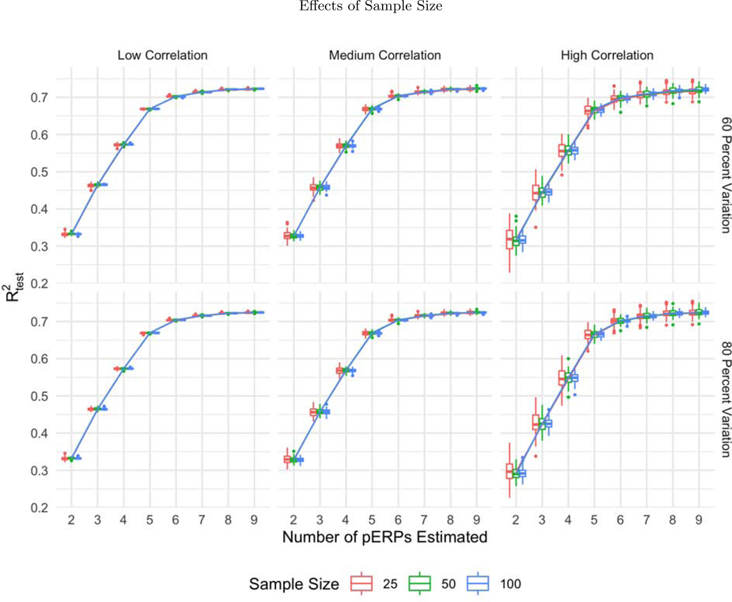
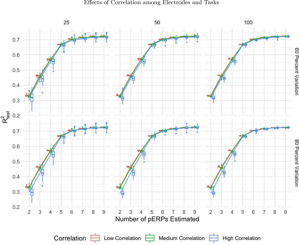
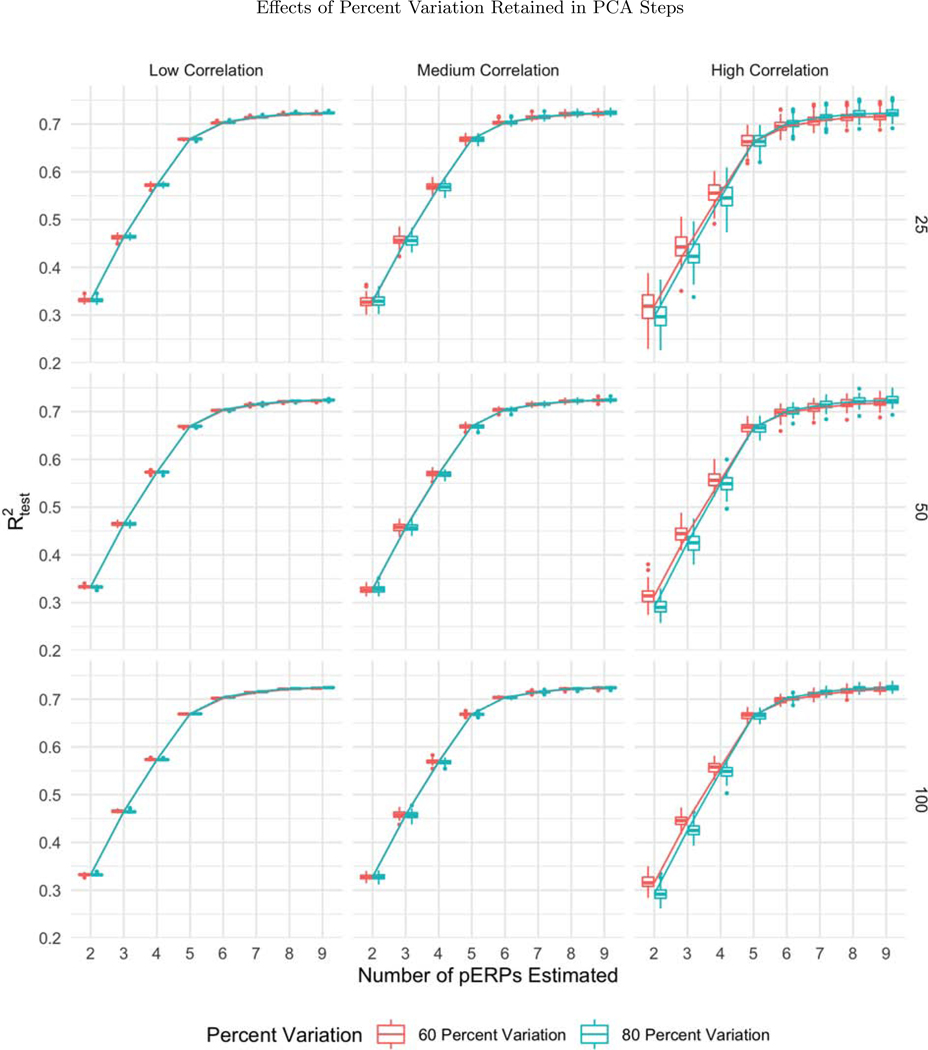
While all three sample sizes considered provide sufficient information for recovery of the records (with steady $R_{\text{test}}^2$ levels across sample size), the variability in prediction accuracy decreases with increasing sample size, as expected, depicted in the narrower boxplots for larger N in Figure 5. Since higher correlations across electrodes and tasks correspond to smaller effective total number of records, the prediction accuracy gets worse (with greater variability) as depicted in Figure 6. The percent of variation retained for PCA does not appear to affect the $R_{\text{test}}^2$ except for the high correlation case. When the correlation among electrodes and tasks is high, retaining more variation in PCA corresponds to retaining more noise, since repetitions over tasks and electrodes look more similar, leading to worse prediction accuracy (Figure 7).

Figure 5:

The boxplots of $R_{\text{test}}^2$ as a function of the number of pERPs estimated across 100 simulations with 60 (first row) and 80 percent variation retained (second row) and low (first column), medium (second column) and high (third column) correlation between electrodes and tasks for N = 25 (red), 50 (green), and 100 (blue). The variability in prediction accuracy decreases with increasing sample size, as expected.

Figure 6:

The boxplots of $R_{\text{test}}^2$ as a function of the number of pERPs estimated across 100 simulations with 60 (first row) and 80 percent variation retained (second row) and N = 25 (first column), 50 (second column), and 100 (third column) for low (red), medium (green) and high (blue) correlation between electrodes and tasks. With increasing correlation, we see increasing variability in prediction accuracy.

Figure 7:

The boxplots of $R_{\text{test}}^2$ as a function of the number of pERPs estimated across 100 simulations with N = 25 (first row), 50 (second row), and 100 (third row) and low (first column), medium (second column) and high (third column) correlation between electrodes and tasks for 60 (red) and 80 (blue) percent variation retained. When the correlation is high, retaining more variation in PCA corresponds to retaining more noise, leading to worse prediction accuracy.

Method Comparisons

The pERP-RED algorithm is compared to three different sets of basis expansions: Fourier, functional principal component analysis (FPCA), and a set derived using a single PCA and ICA similar to pERP-RED. Using Fourier bases, many more components are required to achieve the same predictive accuracy (see Supplementary Figures 4 through 7). This is expected, because these bases are fixed ex ante rather than being data-derived. The other three methods, all deriving their bases from the data, produce very similar prediction accuracy in terms of both $R_{\text{test}}^2$ and $R_{\text{pERP}}^2$ values (plots deferred to the supplementary materials). Additionally, a central feature of the pERP-RED approach is that the estimated bases are chosen not arbitrarily or ex ante but rather to describe the variation that was important to the original data structure. Consequently, as demonstrated in our applications, the non-arbitrary nature of these basis leads to substantive interpretations of the processes they may be detecting.

The difference between pERP-RED and FPCA is the ICA step employed by pERP-RED, which arises due to a conceptual difference in what information they seek to extract. FPCA chooses the bases that will explain the greatest variation in the data with the fewest components. By comparison, pERP-RED follows a similar logic in the initial reduction steps then employs an ICA in the final step because, as in other blind source-separation problems, maximizing the independence (not just orthogonality) of the components is a means to extract maximally “unmixed” underlying signals. These two approaches are expected to explain similar amounts of variation in the data, but the latter adds greater value to the intended interpretation of their pERPs. As expected, our simulation shows very similar values for $R_{\text{pERP}}^2$ and $R_{\text{test}}^2$ in the two methods, with FPCA having a slightly lower $R_{\text{pERP}}^2$ (Supplementary Figures 4 and 5) and pERP-RED having slightly lower $R_{\text{test}}^2$ (Supplementary Figures 6 and 7).

As a final comparison, we consider a variation of pERP-RED we will call “single-PCA”, where there is only one data concentration (PCA) step and one ICA step. The single PCA would be conducted on the matrix formed by using all of the subjects and electrodes in the columns. We see in simulations (Supplementary Figures 4 through 7) that the pERP-RED and the “single-PCA” method perform similarly in terms of signal recovery in this setting on values of $R_{\text{pERP}}^2$ and $R_{\text{test}}^2$. However the two have important differences in practice. First, the single-PCA method is limited in that the number of subjects times electrodes cannot exceed the number of time points times tasks because the PCA step would fail without additional constraints. The pERP-RED approach does not have this limitation, since the first PCA will reduce the number of electrodes before multiplying by the subjects. Second, by separately doing the electrode reduction within subject, pERP-RED allows subjects to vary arbitrarily in their electrode topography (and missingness), the projections of sources onto those electrodes, and the subject-specific components for their weightings. By contrast, the “single-PCA” reduction effectively assumes homogeneity in all these features across subjects. Lastly, pERP-RED allows the user to control the amount of variation used in each PCA step separately if they deem appropriate.

4. Applications

4.1. ASD Study

The first application of pERP-RED examines EEG data from a study of the neural mechanisms underlying language impairment in children with Autism Spectrum Disorder (ASD) (DiStefano et al., 2019). This group has been difficult to study using traditional paradigms that require following instructions or providing behavioral responses. Thirty-one children, aged 5–11 years old, who participated in the below described paradigms and provided sufficient high quality EEG data were considered: 14 typically developing (TD), 10 verbal ASD (vASD), and 7 minimally verbal ASD (mvASD). The three groups were age-matched. In the ASD participants, diagnoses had been made prior to enrollment, through clinical diagnosis by independent clinical psychologists, child psychiatrists, and/or developmental pediatricians. These diagnoses were confirmed by the research team using the Autism Diagnostic Observation Schedule (ADOS) and Social Communication Questionnaire (SCQ).

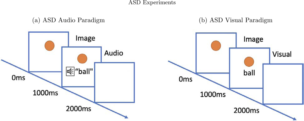
Two picture-word matching paradigms were used, one audio and one visual. The word stimuli included 60 basic nouns taken from the MacArthur-Bates Communicative Development Inventories-2nd edition. Examples of words included animals such as a bird or a dog and inanimate objects such as a doll or a bike. In the audio paradigm, a picture of the word would appear on a white background and the child would hear a spoken word that was either the same (match condition) or a word neither semantically nor phonologically matched the word image (mismatch condition). In both conditions, the picture image appeared for 2000ms, where the auditory stimulus was played after 1000ms after the picture image was shown (see Figure 8). Each word image pair appeared twice—once in the matched and once in the mismatched condition. No behavioral response was required. Trials were presented in four blocks of 30 trials each, totaling 6 minutes.

Figure 8:

In both paradigms, the image appears for the full 2000ms. (a) In the audio paradigm, a spoken word is heard 1000ms after the onset of the image. (b) In the visual paradigm, the word image is seen 1000ms after the onset of the image.

The visual paradigm used the same nouns and same number of trials, but in each an image of the word appeared on screen after 1000ms rather than an audio recording (see Figure 8). As in the auditory paradigm, the two conditions are “match” or “mismatch”. In both paradigms, the trials were video recorded in order to remove trials in which the participants were not looking at the screen. Data collection, cleaning, and pre-processing steps are described in the Appendix.

Results for ASD study

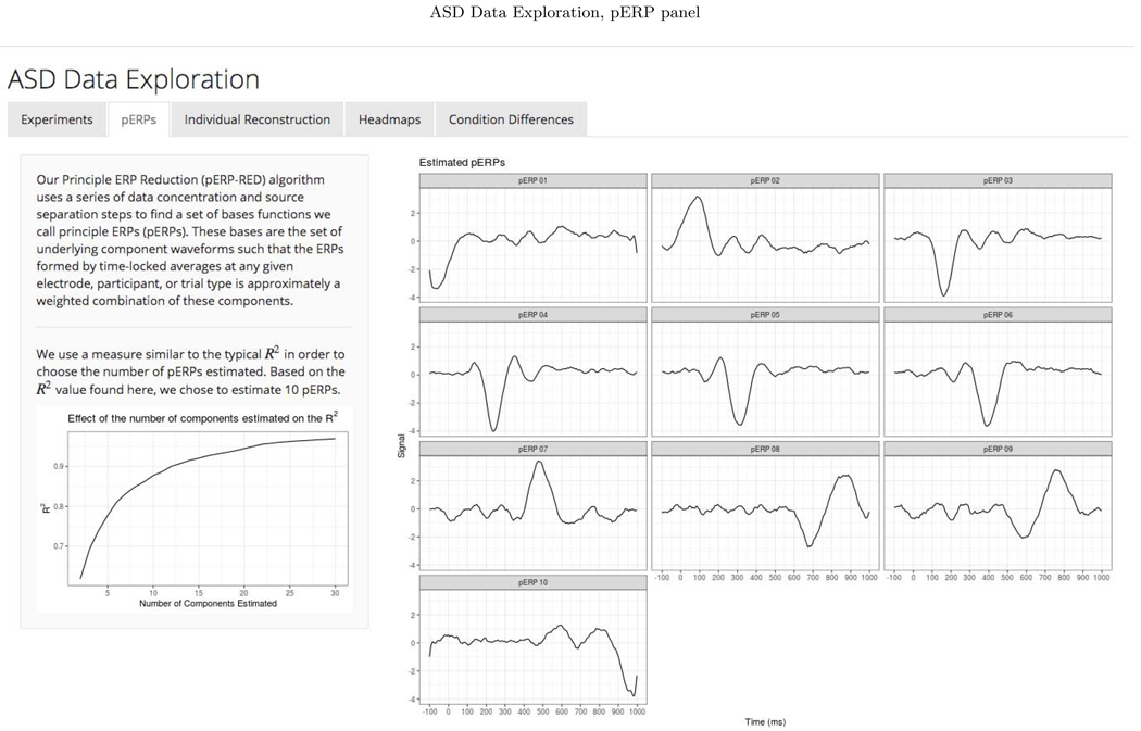
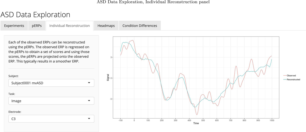
We chose to retain enough components to explain 90 percent of the total variation in the PCA steps of the pERP-RED algorithm. To choose an appropriate number of pERPs, we estimated the pERPs using P = {2, 3,...,30} and the total computing time was approximately 4 minutes when parallelized on a 2.4 GHz 6-Core Intel Xeon processor operating R 3.6.2 (R Core Team, 2019). Ten pERPs achieve an R² value of 0.89 and are given in Figure D.1 ordered by their peak locations. We regress each demeaned record (subject and electrode ERP from each task), denoted by Y_j, on the set of estimated pERPs, Φ, to obtain the corresponding coefficients, ω_j. These coefficients can be used to reconstruct a less noisy version of each record as is shown in Appendix Figure D.2. To enhance transparency and encourage exploration of this approach, we provide a user-friendly data browser (ASD Data Exploration, https://perpred.shinyapps.io/asd_exploration/), where all analysis described here and others can be reproduced through a graphical interface. The user can thus become acquainted with the method before applying pERP-RED in their own lab. Screenshots from the application, providing graphics that mirror those used here, are provided in Appendix D.

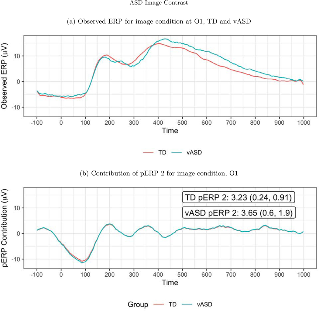
To investigate the spatial distribution of pERP loadings, headmaps can be used to plot the estimated coefficients (averaged over all subjects) across the scalp as Figure D.3 shows for the image task. The coefficients of the first two pERPs are loaded heavily onto in the O1 and O2 electrodes. Notably, the overall ERP waveform from the image task (Figure 9, top) does not look as might be expected, showing no evidence of an N1 due to visual activation. However, our approach explains why the waveform does not include a negative deflection consistent with the N1 component, and recovers the ability to analyze the amplitude of a “hidden” component resembling the expected N1. Specifically, the time course of pERP 1 shows ongoing activity from the prior trial in the −100 to 0 ms interval. Such temporal overlap is to be expected given the fast rate of trials and that the ITI was fixed rather than jittered. However, the time course of pERP 2 is akin to the expected N1, peaking negatively around 90ms. The observed overall waveform, receiving contributions from both pERP 1 and 2, shows a relatively flat signal from −100 to 100ms. Figure 9 shows the contribution of pERP 2 to the overall waveform, in the TD and vASD groups. Loadings on pERP 2 are significant in all diagnostic groups, as would be expected for a visual task, and do not show significant group differences. However, the variation in loadings across participants, indexed by the APSD, is 60% higher for the vASD group than for the TD group. Such higher variation in the vASD than TD group is generally to be expected. This is an important example of where the pERP-RED and pERP-space analysis is useful: Supposing the N1 indexed important activity we wish to measure for research or clinical purposes, it would have been ineffective to have measured it in this particular experiment using a peak or mean negativity around 100ms. Yet, a component resembling the N1 was elicitetd and can be indexed using the coefficient on pERP 2. This component shows similar average magnitude in the TD and vASD groups, but far greater variability in the latter.

Figure 9:

(a) The observed average ERP waveform for the image condition, by group. No N1 is evident. (b) ERP reconstructed using only pERP2, i.e. pERP 2 scaled by its contribution to the waveform (O1 plotted here). This component is detected despite the apparent lack of an N1 in the overall ERP because we also identify and model pERP 1, which captures spillover from the prior trial. The numbers shown are the mean weight with SE, and APSD in parentheses. The APSD reflects the subject variability and is much larger in the vASD group. Thus the vASD group has an average response very similar to that of the TD group, but there is a great deal more variability in the vASD group.

As noted, this approach also makes it easy to examine all pERPs for their loadings or significant differences in contrasts. While increasing the number of comparisons, this is done without user discretion of the sort allowed by user-driven selection of time intervals. For the image task, in addition to the expected N1 component that is recovered by this method, significant coefficients for pERPs 6 and 7 are found at O1 and O2, peaking positively around 450ms. This late positivity, present in all diagnostic groups, may be related to anticipation of the next stimulus. No other pERPs showed loadings that were statistically distinguishable from zero at these locations.

In the visual paradigm, the largest loadings are observed for pERP 7 across diagnostic groups found in the frontal and central regions (electrodes F3, F4, FZ, C3, CZ), corresponding to a negativity observed around 500ms. For loadings onto pERP 7, the mismatch condition was associated (though not significantly) with a stronger negativity than the match condition, as expected, in the TD group (possibly related to greater semantic processing).

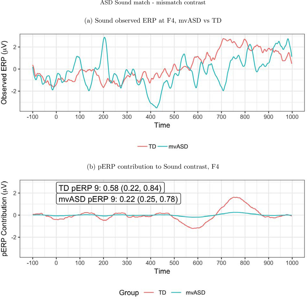
For the auditory paradigm, a significant group difference emerges frontally at electrode F4, in pERP 9 when comparing activity between the TD and mvASD groups in the contrast of match vs. mismatch conditions (Figure 10). In the TD group, the mismatch condition leads to a deeper negativity than the match condition, seen around 700–800ms. This late negativity, expected to be larger in the mismatch condition, has been linked to semantic integration in the previous work of DiStefano et al. (2019).

Figure 10:

(a) ERP waveforms at F4. (b) A significant difference was found on pERP 9 between the mvASD and TD groups when contrasting match vs. mismatch. The numbers reported in the figure are the mean, with the SE and APSD in parentheses. This echoes a previously reported finding that the mismatch condition led to a deeper negativity at 700–800ms, thought to reflect semantic integration.

The prior work of DiStefano et al. (2019) study only the audio paradigm, and not the visual paradigm. Their main findings include a deeper negativity for mismatch than match trials, which they label as both an N4 and a later negativity, similar to the pERP 9 component picked up by the pERP-RED analysis. In relation to the N4, we see “N4-like” pERPs (5 and 6), peaking around 300 ms and 400 ms respectively. At Pz for example, we see the expected deeper negativity on these two pERPs for mismatch than for match trials, in each group. In the TD group, this difference in the amplitudes is large and statistically significant for pERP 5 (t = 2.1) though less so for pERP 6 (t = 1.4). In the vASD and mvASD, the differences appear similar but miss significance, ranging from t = 1.4 to t = 1.8.

Relatedly, we also notice pERP 4, which peaks slightly earlier around 240 ms. This component also generates a significantly deeper negativity for mismatch than match in the TD group (t = 2.1) and in the mvASD group (t = 3.0), but interestingly shows no difference in the vASD group (t = 0.1). This is consistent with a finding in DiStefano et al. (2019) that perhaps surprisingly, mvASD participants appear more similar in many ways to TD than does the vASD group. Further, the vASD group may have far greater heterogeneity than the others: the APSD values for pERP 4, are on the order of 0.5–0.7 for the match and mismatch conditions in both the TD and mvASD groups, but are 1.2 (match) and 1.6 (mismatch) in the vASD group. That is, the standard error of coefficients across participants in the vASD group is 2–3 times larger than in TD or mvASD groups, again echoing the heightened heteregoeneity of the vASD groups noted in DiStefano et al. (2019).

4.2. ADHD Study

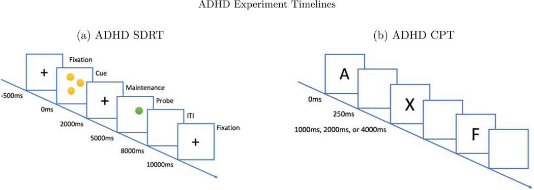
We also test the methods on a dataset that is larger in terms of participants, diversity of tasks, and electrodes: a study of cognitive control in youth, aged 7–17 years old, with and without Attention Deficit and Hyperactivity Disorder (ADHD) with N = 331, of whom N_ADHD = 242 are in the ADHD group (clinicaltrials.gov ID: NCT00429273). Additional methodological details can be found in Lenartowicz et al. (2019). We examined data pooled from two sets of tasks: a spatial delayed response task (SDRT), and a continuous performance task (CPT) (see Figure 11). In the SDRT, participants are instructed to pay attention to the location of yellow dots on the screen against a black background. Each trial consists of a 500 ms fixation cross, followed by the yellow stimulus dots for 2000 ms (cue). Subjects are presented varying memory load of 1, 3, 5, or 7 dots at a time, in random order. Then a blank screen with a fixation cross appears for 3000ms (maintenance phase). Finally, a single probe green dot is presented for 3000ms (retrieval phase), during which the participant indicates whether the position of the probe matched the position of any of the yellow dots (pressing the left arrow to indicate a match, the right arrow to indicate a non-match). On half of the trials the green dot matched the location of a yellow dot and on half it did not. The trial ends when the participant responds, after which a fixed 3000 ms ITI (a blank screen) is displayed. If no response is made during the 3000 ms response interval, a message appears indicating that the subject did not respond and the next trial begins. Subjects are required to score above 50% accuracy on a series of practice rounds in order to move on to experimental blocks. There are 48 trials in each experimental block, and 2 blocks, with equal numbers of load sizes and equal numbers of match and no-match trials. Total experimental time is about 7 minutes per block, 14 minutes total. Including the training and practice trials the entire task requires roughly 17 minutes. ERPs are time-locked to cue, to probes, and to participant responses.

Figure 11:

(a) In the SDRT task, a sequence of screens are presented. A fixation cross for 500ms, the cue dots for 2000ms, another fixation cross for 3000ms, and the probe dot for 3000ms. Within the 3000ms probe phase, the subject responds. (b) In the CPT task, the subject is presented with either an ‘X’ or ‘not X’ for 250ms, after which there is a blank screen for either 1000, 2000 or 4000ms before the next trial.

The CPT requires sustained attention (or vigilance) and response inhibition. Subjects are presented single letters (A, B, C, D, F, I, L, O, T, or X), one at a time in the center of the computer screen. The subject is instructed to press and release the spacebar as quickly as they can after viewing each letter – except when the letter is “X”, which indicates they should make no response. There are 360 continuous trials randomly presented with three different ISI lengths: 1000, 2000, or 4000 ms. Each letter is always presented for 250 ms, leaving either 750, 1750, or 3750 ms of remainder response time per trial, see Figure 11. Epochs are time-locked to stimulus onset. For present purposes, we categorize trials into just four types based on combinations of the cue (“X” or “not X”) and response (“correct” or “incorrect”), Table 1. Data collection, cleaning, and pre-processing steps are described in the Appendix.

Table 1:

ASD and ADHD Tasks and Trial Types

We consider 5 separate trial types/ tasks drawn from the two ASD experiments (Audio and Visual). From the two ADHD experiments (SDRT and CPT), we consider 8 separate trial types/tasks.

ASD		ADHD
Image	Visual Match	SDRT Cue	CPT X Correct
Audio Match	Visual Mismatch	SDRT Probe	CPT X Incorrect
Audio Mismatch		SDRT Response Correct	CPT Not X Correct
		SDRT Maintenance	CPT Not X Incorrect

No other results from the CPT task of this dataset have been published as yet. For the SDRT, Lenartowicz et al. (2019) describes a number of results, focusing principally on spectral EEG analyses, and particularly alpha modulation during the encoding and maintenance stages as a predictor of impairment. This study did however index vigilance using the P2 event-related potential in response to the onset of the fixation, finding a nearly-significant smaller P2 in the ADHD group compared to the TD group at FCz.

Results for ADHD study

To choose an appropriate number of pERPs, we estimated the pERPs using P = {2, 3,...,30} and the total computing time was approximately 43 minutes when parallelized on a 2.4 GHz 6-Core Intel Xeon processor operating R 3.6.2 (R Core Team, 2019). The computation time is longer compared to the ASD analysis due to the larger sample size. Fifteen pERPs achieve an R² value of 0.88 and will be used in the analysis. While the SDRT and CPT data are too rich to fully examine here, we consider a number of analyses that illustrate the pERP approach. The CPT data cannot be made public as yet, but all analyses of the SDRT described here can be replicated using our online data browser (https://perpred.shinyapps.io/adhd_exploration/). In comparison to Lenartowicz et al. (2019), at FCz we do not see significant evidence for a difference between the ADHD and TD groups on a P2-like component following the fixation’s onset. However, if the ADHD and TD groups differ in vigilance to task relevant stimuli, we might expect to see this not only in the P2 to fixation, but in components such as the N1 and P2 following the encoding cue itself. Continuing to look at FCz, we do see pERPs reflecting an apparent P2 (pERP 5, a positive peak near 200 ms post encoding cue), and the N1 (pERP 4, a negative peak near 130 ms). Both show significantly non-zero loadings in the expected directions, for both ADHD and TD groups. While the differences in these average loadings (for ADHD vs. TD groups) do not reach statistical significance, the TD group shows a marginally larger loading on the N1-like component (pERP 4) with a t-statistic of 1.2 for the comparison. We consider the N1/P2 more extensively below.

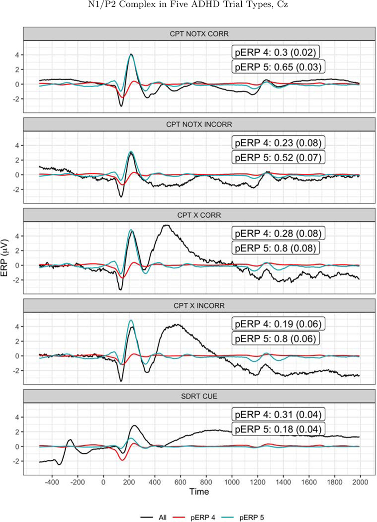
There is a great deal more to report from this dataset, and we focus here on analyses that aid in evaluating the validity or usefulness of a pERP-based approach. First, as a validation exercise, we test the degree to which the algorithm identifies a N1/P2 complex in both the CPT and SDRT tasks. The N1/P2 complex has been widely identified in tasks involving visual stimuli and attention, such as the CPT and SDRT. If our approach is effective in constructing pERPs that reflect important or common sources of variation, having pooled both the CPT and SDRT to construct those pERPs, we might expect to see such components. Figure 12 shows the two pERPs noted above that appear to correspond to a N1 (pERP 4) and P2 (pERP 5), though the latter also contains a small negative deflection prior to 200ms. In the CPT experiment, taking Cz as an example, all four (visual) stimulus-locked trial types (X(No Go)-correct, X(No Go)-incorrect, notX(Go)-correct, notX(Go)-incorrect) show weights on pERPs 4 and 5 that are distinguishable from zero significantly, suggesting that the four trials types elicitetd pERPs 4 and 5 as would be expected. Furthermore, as shown in Figure 12, in each of the CPT trial types, the reconstructed signal using just these two components reproduce the expected form of a N1/P2 complex following the visual stimulus. The same holds for the all of the cue-locked trials of the SDRT experiment, and not for the response-locked or probe-locked trial types.

Figure 12:

The N1/P2 as observed (solid black line) and as reconstructed from pERPs 4 (red line) and 5 (blue line) at CZ, at each of the five trials types. The loadings and standard errors for those loadings is shown in each figure. The corresponding t-statistics (mean divided by SE) range from 2.9 to 22 across these 10 cases, leading to firmly to rejecting the null hypothesis (of zero loading) in each.

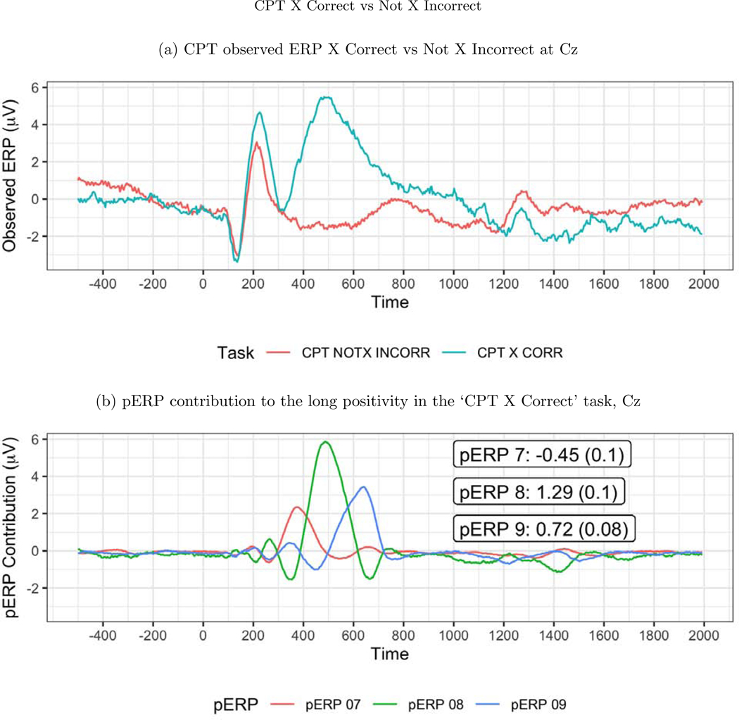
Next we turn to task specific expectations to further probe the validity of the approach. In the CPT task, trials with an “X (No Go)” are relatively rare, and are thus expected to produce an update or novelty signal typically associated with the P3. We thus expect to see activity at 300–500ms in a contrast of “Not X (Go)-incorrect” versus “X (No Go)-, correct” in central and frontal areas. We contrast these two trial types because neither contain motor activity due to the response. Indeed, the observed ERP waveforms show a large positivity in the “X (No Go)-correct” trials, and not in the”Not X (Go)-incorrect” trials at sites such as Cz, see Figure 13 (top). This large difference between these two waveforms is quite broad, perhaps containing more than just a conventional P3, or averaging together positive deflections that peak at varying latencies. The estimated pERPs support such a hypothesis: We see that this contrast is explained not by a single broadly shaped pERP, but by pERPs 7, 8, and 9. These three pERPs each show a relatively sharp positivity, but at different latencies: 375ms for pERP 7, 475ms for pERP 8, and 625ms for pERP 9, see Figure 13 (bottom). In fact, all trial types with an “X” (i.e. No Go trials) regardless of response show heavy loadings on these three pERPs, whereas trial types without an “X” (and thus the majority stimulus type), regardless of response, show little weight on these pERPs, consistent with the expectation that pERPs 7, 8, and 9 relate to an updating or novelty or updating signal. As these three components have different latencies, they combine to form the slower peaking positivity seen in the overall waveform.

Figure 13:

(a) The observed ERP at Cz. The ‘X Correct’ and ‘Not X Incorrect’ tasks are used for this contrast because neither include a motor response. The large positivity in the ‘X Correct’ task is expected as it indicates the update/novelty of seeing a rare event. (b) The large positivity in the ‘X Correct’ task from 400–800ms can be decomposed into pERPs 7 (red), 8 (green), and 9 (blue). The numbers shown are the mean and SE of the coefficients.

This highlights a potential use for such decompositions as compared to examining mean/peak amplitudes in the superposed ERP alone. Investigators could use the loadings on each of these three components, at the individual or group level to see if individual differences in clincial diagnosis or task performance correspond to different coefficients on these three novelty-related pERPs. In this case, the coefficients and their contrasts on these three pERPs are remarkably similar at least across the ADHD and non-ADHD groups. They also do not systematically vary as a function of participant age. Whether these individual, low-dimensional scores are more informative or predictive (of other behaviors, symptomology, or other traits) than a simple mean amplitude over some interval or a measure of latency remains an interesting question for the next phase of research with pERPs.

Turning to the SDRT task, we take the opportunity to illustrate another use of the pERP approach: characterizing heterogeneity. In addition to the standard errors that are used for inference, we provide the “across participant standard deviations” (APSD), which characterize how the loadings on a given pERP vary from one participant to the next. Consider, for example, the waveform for the maintenance period in the SDRT. Because ADHD has implications for the ability to maintain attention and working memory resources on task, we may expect differences here. Table 2 shows loadings for all pERPs in the maintenance condition at electrode Cz, separately for typically developing (TD) participants and those categorized as either ADHD-inattentive or ADHD-combined (containing participants diagnosed with both inattention and hyperactivity). On the loadings, we see larger differences between the TD group and the ADHD-combined group, though these do not reach statistical significance³, while the TD and ADHD-inattentive group tend to be more similar. Returning to the question of heterogeneity, the TD and ADHD-inattentive group have very similar levels of heterogeneity in loadings, as indicated by the APSD value on each pERP. By contrast, the ADHD-combined group has higher APSD values on every pERP, indicating greater heterogeneity across the individuals that make up this group. Heterogeneity is especially large in the first two pERPs, and again for pERPs 10–13 onward. The early pERPs 1 and 2 appear to reflect activity before the cue has disappeared from the screen, while pERPs 10–13 contribute to a late ongoing positivity in the waveform — perhaps related to maintenance of task-relevant attention or working memory.

Table 2:

ADHD and TD Groups: SDRT Maintenance Condition (Cz)

The APSD captures variability across participants in the weight given to each pERP. We see that the ADHD group has a much higher APSD for many of the pERPs than the TD group.

	Combined			Inattention			TD
pERP	Mean (SE)	t	APSD	Mean (SE)	t	APSD	Mean(SE)	t	APSD
pERP 01	−0.11 (0.27)	−0.41	2.94	0.32 (0.14)	2.30	1.50	0.41 (0.15)	2.67	1.44
pERP 02	0.18 (0.28)	0.65	3.01	−0.29 (0.15)	−1.91	1.68	−0.41 (0.18)	−2.28	1.69
pERP 03	0.1 (0.18)	0.58	1.91	−0.11 (0.13)	−0.86	1.41	−0.32 (0.15)	−2.10	1.44
pERP 04	0.02 (0.1)	0.23	1.07	0.09 (0.09)	1.06	0.94	0.22 (0.1)	2.25	0.90
pERP 05	0.21 (0.11)	1.96	1.15	0.1 (0.08)	1.17	0.90	−0.02 (0.09)	−0.20	0.87
pERP 06	0.13 (0.11)	1.22	1.17	0.07 (0.09)	0.81	0.94	0.08 (0.1)	0.86	0.90
pERP 07	0.28 (0.12)	2.30	1.29	0.35 (0.09)	3.80	1.02	0.45 (0.09)	4.89	0.86
pERP 08	−0.13 (0.12)	−1.03	1.34	−0.14 (0.09)	−1.66	0.94	−0.31 (0.1)	−3.11	0.93
pERP 09	0.07 (0.15)	0.51	1.56	−0.01 (0.07)	−0.12	0.79	−0.07 (0.09)	−0.80	0.80
pERP 10	−0.17 (0.17)	−1.02	1.83	0.04 (0.08)	0.54	0.88	−0.03 (0.08)	−0.43	0.74
pERP 11	−0.01 (0.11)	−0.11	1.18	−0.04 (0.06)	−0.69	0.70	−0.06 (0.07)	−0.82	0.68
pERP 12	0.09 (0.14)	0.64	1.55	−0.08 (0.06)	−1.29	0.65	−0.04 (0.06)	−0.73	0.56
pERP 13	−0.08 (0.18)	−0.45	1.97	0.09 (0.08)	1.07	0.91	0.13 (0.11)	1.18	1.07
pERP 14	−0.07 (0.15)	−0.48	1.56	0.1 (0.11)	0.90	1.25	0.11 (0.11)	1.02	1.01
pERP 15	−0.26 (0.19)	−1.37	2.01	0.16 (0.13)	1.23	1.42	0.14 (0.15)	0.96	1.38

Using the pERP-space approach has several benefits over picking an interval, computing a mean or peak amplitude by subject, and compare the standard deviations across those measures by group. First, it seeks to mitigate the overlap problem that is inherent in using peak/mean amplitude, which sometimes makes peaks of important components difficult or impossible to locate, as in the N1 example in the ASD data above. Second, it avoids the requirement of picking the interval over which to do this, and thus reduces the risk of over mining the data to find an interval that works. Third, the pERP-space approach pinpoints variability in terms of the pERPs involved rather than a broad interval. By doing so, it suggests which pERPs show most variability and would thus be interesting to examine at the individual (or even trial-by-trial) level to compare against behavior or diagnostic status.

5. Discussion

We describe a method for estimating an underlying set of components and then analyzing ERP waveforms in terms of these components. The fundamental idea is that any ERP waveform, from any electrode, subject, condition, and task, can be represented as a weighted combination of an underlying set of waveforms. The pERP-RED algorithm provides one reasoned approach to empirically estimate an underlying set of components (pERPs) from a corpus of ERP data, taken across participants and tasks. We then describe how investigators can use these pERPs to extract information from the ERP waveform. To ensure the accessibility of this approach, we provide software that enables users to import ERP waveforms, estimate pERPs, and conduct the pERP-space analyses described in this paper (the pERPred package in R).

This approach has many advantages relative to the standard practice of extracting the mean or peak amplitude in a user-specified window and presuming the result indexes the magnitude of a known ERP component of ex ante interest. First and foremost, it sidesteps the long-standing concern that differences observed at a particular interval may be due to a component other than that of interest. It similarly addresses concerns of spillover from the prior trial. As a result, this approach not only dissociates the measurement of components from the measurement of peaks, but can measure components that don’t even visibly appear as a peak in the waveform due to overlap (as in the N1 in the ASD example above). It can also show that one broad slow-peaking structure may be explained as a combination of multiple underlying components, each of which can be measured on the group or individual level (as for the P3 in the ADHD example above). The ability to measure the contribution of every pERP contributing to the observed waveform, for each group or individual, makes the pERP approach particularly relevant to investigators seeking to discover biomarkers from group or individual level data. Relatedly, the pERP-space approach is useful for characterizing heterogeneity across individuals in a given group, assessing the variation of the relative contributions of every pERP for every participant via the APSD score we provide.

An additional advantage relates to broader research practice in terms of selective reporting and discovery. Our approach employs multiple comparisons, but the number of hypotheses that will be tested (at least at a given electrode and for a given contrast) is simply the number of pERPs, and can be accounted for through any multiple comparison correction the user would like. Investigators can transparently report all significant and non-significant results for a given condition or contrast, characterizing (non) differences in any pERP, and thus over the entire time course. By contrast, in standard practice, the user chooses the time interval(s) and reports only differences there. Moreover, there is no clear way to exhaust the set of components that may or may not differ in a conventional analysis as can be done in a pERP-space analysis. Our approach facilitates discovery of differences in underlying components not previously of interest, yet avoids a user-driven search for such differences.

A number of areas for future exploration exist, in particular to further probe the validity or test the usefulness of this approach. First, it is natural to extract the weight on a given pERP of interest at the trial-wise level, in order to see how they might predict or relate to trial-wise behavior. This has parallels in recent work on high-dimensional modeling of EEG data. For example, Hasenstab et al. (2015) model longitudinal trends over trials within ERPs from a single learning task. Hasenstab et al. (2017); Scheffler et al. (2020); Fiecas and Ombao (2016); Ombao et al. (2018) consider high-dimensional modeling of EEG including the trial dimension using functional data and time series analysis approaches. While functional data analysis has seen rapid growth over the past two decades, with important recent work modeling multivariate hierarchical functional data (Di et al., 2009; Shou et al., 2015; Happ and Greven, 2018; Zhang et al., 2019), existing works have not considered data structures observed across multiple experiments, groups, subjects, electrodes, tasks and conditions, as we have done in this paper. We consider development of high-dimensional functional principal components decompositions suitable for the complex hierarchical structure considered in this paper as an important direction of future work. Second, a source localization approach conducted on pERPs (as activated in a given task) would be a useful next step. Since its early days (e.g. Makeig et al. 1995) ICA has been proposed as a means of isolating sources that are more likely to represent separate cortical generators and thus be well suited for a source localization step through later dipole modeling. Whereas ICA waveforms for source localization are computed separately on each subject, the fact the pERPs are computed globally on a multi-subject dataset provides new opportunities for seeing how a single pERP localizes, in different subjects, without having to use clustering or other approaches to link components in one subject to those in another. Specifically, the headmap constructed for a given pERP in a given condition can be used as input to a dipole modeling algorithm. It is then an empirical question as to whether a given pERPs activity in a given condition will localize to similar regions in separate subjects. This provides ample opportunity for falsification, since nothing in the algorithm constrains the spatial distribution of a pERP to be similar across participants.

Finally, we want to point to several limitations of pERP-RED. First, pERP-RED can only accommodate data in which the product of the total number of time points and the total number of tasks exceeds the number of all principal regions across all subjects (derived in the first PCA step of electrode reduction). This limitation is a by product of the second PCA step of subject, region reduction in pERP-RED. This condition was satisfied in both data applications. A second limitation is that the derived pERPs are not penalized in time to attain a desired degree of smoothness. Related to the functional data analysis approaches mentioned above that would consider the structure along the time dimension, an interesting direction of future work would be to also consider penalization in time such as localized PCA (Chen and Lei, 2015) which can set estimated basis functions to zero in time windows of little variation, further enhancing interpretation of the derived pERPs.

Appendix A. Supplementary data

Supplementary data including additional figures referred to in Section 3 can be found online with this article.

Appendix B. ASD data collection and pre-processing

EEG was ecorded at 500 Hz using a 128-channel HydroCel Geodesic Sensor Net. Prior to EEG data cleaning, the electrodes were interpolated and reduced to 25 in EEGlab by spherical interpolation (Perrin et al 1989) using the function eeg interp. EEG was digitally filtered using a 0.3 to 30 Hz bandpass filter, segmented into 1000 ms epochs starting at 100 ms before the stimulus (picture, audio or word) onset, and baseline corrected using mean voltage during the 100 ms pre-stimulus baseline period. An automatic artifact detection tool was used to reject electrodes with amplitude difference (max-min) greater than 150mV, usually due to excessive electrode movement, or movement of the cap. Following this automatic artifact detection, each trial was visually inspected to remove any remaining channels that contained EMG, eye-blink, or eye-movement artifacts from further analysis. Trials with more than 15% bad channels were rejected. Only subjects with more than 10 artifact-free trials per condition were accepted for further analysis. For pERP-RED analysis, ERPs averaged over trials, time-locked to the picture onset, the auditory stimulus, and the word image for both match and mismatch conditions are considered producing 5 trial types: image, sound match, sound mismatch, text match, and text mismatch. Epochs considered for pERP-RED were restricted to −100 to 1000ms.

Appendix C. ADHD data collection and pre-processing

Recording and pre-processing details are similar to those reported in Lenartowicz et al. (2019). All recordings were collected with a 40 channel Electrocap with electrodes positioned as in the 10/20 system. Impedences were reduced to 10 KΩ before recording on MANSCAN hardward and software. Continuous EEG was collected at 256 Hz, referenced by linked mastoids. Pre-processing of data was done using EEGLAB software (v.11.03.b, Delorme and Makeig 2004). Data were high-pass filtered at 0.1 Hz. Noisy electrodes (determined by visual inspection) were removed from further analysis. In each subject, epochs with movement or muscle artifacts were identified and removed if signal power in that epoch exceeded the 85th percentile for > 60% of the channels. The resulting continuous data were then epoched and averaged per subject to arrive at the ERPs used in the main text. Epochs considered for pERP-RED were restricted to −500 to 2000ms.

Appendix D. Online Application for Exploring Results

Figure D.1:

In the ASD Data Browser, there is a panel that displays the estimated pERPs as well as the plot of the $R_{\mathit{\text{test}}}^2$ used to determine the number of pERPs.

Figure D.2:

Each individual observed ERP can be reconstructed using the weights calculated using regression.

Figure D.3:

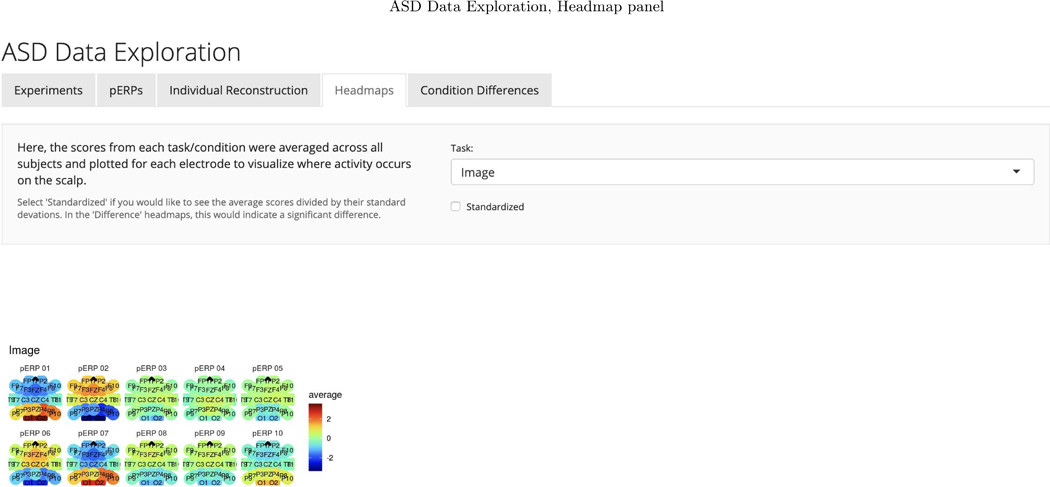
Headmaps can be created in order to visualize where the pERPs are being seen across the scalp. In this case, it can be seen that pERPs 1, 2, 6, and 7 are loaded onto heavily for the Image task.

References

- Chen K. and Lei J. (2015). Localized Functional Principal Component Analysis. Journal of the American Statistical Association, 100(511):1266–1275. [DOI] [PMC free article] [PubMed] [Google Scholar]
- Cong F, He Z, Hämäläinen J, Leppänen PH, Lyytinen H, Cichocki A, and Ristaniemi T. (2013). Validating rationale of group-level component analysis based on estimating number of sources in EEG through model order selection. Journal of Neuroscience Methods, 212:165–172. [DOI] [PubMed] [Google Scholar]
- Delorme A. and Makeig S. (2004). EEGLAB: An open source toolbox for analysis of single-trial EEG dynamics including independent component analysis. Journal of Neuroscience Methods, 134(1):9–21. [DOI] [PubMed] [Google Scholar]
- Di CZ, Crainiceanu CM, Caffo BS, and Punjabi NM (2009). Multilevel functional principal component analysis. Annals of Applied Statistics, 3(1):458–488. [DOI] [PMC free article] [PubMed] [Google Scholar]
- DiStefano C, Şentürk D, and Jeste SS (2019). ERP evidence of semantic processing in children with ASD. Developmental Cognitive Neuroscience, 36:100640. [DOI] [PMC free article] [PubMed] [Google Scholar]
- Eichele T, Rachakonda S, Brakedal B, Eikeland R, and Calhoun VD (2011). EEGIFT: Group Independent Component Analysis for Event-Related EEG Data. Computational Intelligence and Neuroscience, page 129365. [DOI] [PMC free article] [PubMed] [Google Scholar]
- Fiecas M. and Ombao H. (2016). Modeling the Evolution of Dynamic Brain Processes During an Associative Learning Experiment. Journal of the American Statistical Association, 111(516):1440–1453. [Google Scholar]
- Happ C. and Greven S. (2018). Multivariate Functional Principal Component Analysis for Data Observed on Different (Dimensional) Domains. Journal of the American Statistical Association, 113:649–659. [Google Scholar]
- Hasenstab K, Scheffler A, Telesca D, Sugar CA, Jeste S, DiStefano C, and Şentürk D. (2017). A multi-dimensional functional principal components analysis of EEG data. Biometrics, 73(3):999–1009. [DOI] [PMC free article] [PubMed] [Google Scholar]
- Hasenstab K, Sugar CA, Telesca D, Mcevoy K, Jeste S, and Şentürk D. (2015). Identifying longitudinal trends within EEG experiments. Biometrics, 71(4):1090–1100. [DOI] [PubMed] [Google Scholar]
- Huster RJ and Raud L. (2018). A Tutorial Review on Multi-subject Decomposition of EEG. Brain Topography, 31:3–16. [DOI] [PubMed] [Google Scholar]
- Kairov U, Cantini L, Greco A, Molkenov A, Czerwinska U, Barillot E, and Zinovyev A. (2017). Determining the optimal number of independent components for reproducible transcriptomic data analysis. BMC Genomics, 18:1–13. [DOI] [PMC free article] [PubMed] [Google Scholar]
- Lenartowicz A, Truong H, Salgari GC, Bilder RM, McGough J, McCracken JT, and Loo SK (2019). Alpha modulation during working memory encoding predicts neurocognitive impairment in ADHD. Journal of Child Psychology and Psychiatry and Allied Disciplines, 60(8):917–926. [DOI] [PMC free article] [PubMed] [Google Scholar]
- Luck SJ (2014). An Introduction to the Event-Related Potential Technique. MIT Press, 2 edition. [Google Scholar]
- Luck SJ and Kappenman ES (2011). The Oxford Handbook of Event-Related Potential Components. Oxford University Press. [Google Scholar]
- Makeig S, Bell AJ, and Sejnowski TJ (1995). Independent Component Analysis of Electroencephalographic Data. In Proceedings of the 8th International Conference on Neural Information Processing Systems, pages 145–151, Denver, Colorado MIT Press. [Google Scholar]
- Ombao H, Fiecas M, Ting CM, and Low YF (2018). Statistical models for brain signals with properties that evolve across trials. NeuroImage, 180:609–618. [DOI] [PubMed] [Google Scholar]
- R Core Team (2019). R: A Language and Environment for Statistical Computing. R Foundation for Statistical Computing, Vienna, Austria. [Google Scholar]
- Scheffler A, Telesca D, Li Q, Sugar CA, Distefano C, Jeste S, and Şentürk D. (2020). Hybrid principal components analysis for region-referenced longitudinal functional EEG data. Biostatistics, 21(1):139–157. [DOI] [PMC free article] [PubMed] [Google Scholar]
- Shou H, Zipunnikov V, Crainiceanu CM, and Greven S. (2015). Structured functional principal component analysis. Biometrics, 71(1):247–257. [DOI] [PMC free article] [PubMed] [Google Scholar]
- Spencer KM, Dien J, and Donchin E. (2001). Spatiotemporal analysis of the late ERP responses to deviant stimuli. Psychophysiology, 38(2):343–358. [PubMed] [Google Scholar]
- Zhang J, Siegle GJ, D’Andrea W, and Krafty RT (2019). Interpretable Principal Components Analysis for Multilevel Multivariate Functional Data, with Application to EEG Experiments. page arXiv: 1909.08024. [DOI] [PMC free article] [PubMed] [Google Scholar]
Associated Data
This section collects any data citations, data availability statements, or supplementary materials included in this article.