Geospatial immune variability illuminates differential evolution of lung adenocarcinoma

Abstract

Remarkable progress in molecular analyses has improved our understanding of the evolution of cancer cells towards immune escape^1–5. However, the spatial configurations of immune and stromal cells, which may shed light on the evolution of immune escape across tumor geographical locations, remain unaddressed. We integrated multi-region exome and RNA-seq data with spatial histology mapped by deep learning in 100 non-small cell lung cancer (NSCLC) patients from the TRAcking Cancer Evolution through Therapy (Rx) (TRACERx) cohort⁶. Cancer subclones derived from immune cold regions were more closely related in mutation space, diversifying more recently than subclones from immune hot regions. In TRACERx and in an independent multi-sample cohort of 970 lung adenocarcinoma (LUAD) patients, the number of immune cold regions significantly correlated with risk of relapse, independently of tumor size, stage and number of samples per patient. In LUAD, but not lung squamous cell carcinoma (LUSC), geometrical irregularity and complexity of the cancer-stromal cell interface significantly increased in tumor regions without disruption of antigen presentation. Decreased lymphocyte accumulation in adjacent stroma was observed in tumors with low clonal neoantigen burden. Collectively, immune geospatial variability elucidates tumor ecological constraints that may shape the emergence of immune evading subclones and aggressive clinical phenotypes.

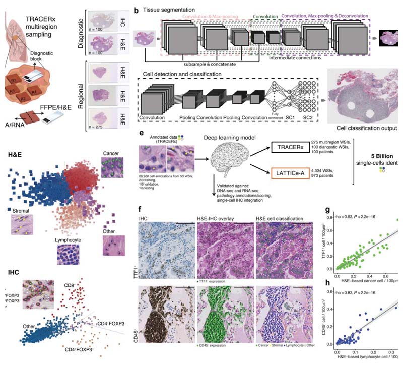
Using an artificial intelligence framework, we developed a generalizable deep learning pipeline to spatially profile immune infiltration and discover tumor topological determinants of immunosuppression in digital pathology. Convolutional neural networks were tailored for the analysis of NSCLC morphology using diverse histology samples in the multi-region TRACERx 100 cohort⁶ to avoid overfitting (Methods). This approach enabled the spatial mapping of cancer cells, lymphocytes, stromal cells (fibroblasts and endothelial cells), and an “other” cell class (macrophages, pneumocytes and non-identifiable cells) in hematoxylin & eosin (H&E)-stained images (275 tumor regions from 85 patients and 100 diagnostic slides from all patients, Fig. 1a-c, CONSORT diagram Extended Data Fig. 1a-b, Supplementary Table 1). T cell subsets were also identified in CD4/CD8/FOXP3 immunohistochemistry (IHC) images for all 100 diagnostic samples (Fig. 1d).

Figure 1. The computational pathology deep learning pipeline for dissecting heterogeneous NSCLC tumor microenvironment.

a. Histology sample generation in Lung TRACERx. To preserve morphology and generate good quality histology, samples from the same tumor regional frozen blocks specifically collected for TRACERx and generated molecular data^1,6 were re-embedded in formalin fixed paraffin (FFPE). From these, H&Estained tumor section slides were generated. In addition, H&E section and triplex CD4/CD8/FOXP3 IHC slides were also generated from diagnostic blocks that represent clinical standard sampling, b. Our multistage deep learning pipeline consists of three key stages: fully automated tissue segmentation, single-cell detection and classification. The final output is shown as an image with all cells identified. For more details, please see the ‘Training the deep learning pipeline’ section of the Methods. c. Illustrative 3-dimensional distribution of input image patches in the feature space learned by the convolutional neural networks, using Principal Component Analysis. The feature clusters were pseudocolored to display segregation for four cell types in H&E, and d CD8⁺, CD4⁺FOXP3⁺, CD4⁺FOXP3^- and “other” cell class (hematoxylin cells) in IHC, respectively, e. The deep learning single-cell classification model was trained using expert pathology annotations from a variety of TRACERx samples (diagnostic, regional, TMA). The trained model was then applied to the remaining TRACERx samples (predominantly LUAD and LUSC) and the LATTICe-A cohort (only LUAD), identifying over 171 million cells in TRACERx and over 4.9 billion cells in LATTICe-A. WSI: whole-section image, f. Biological validation of the deep learning approach. H&E and IHC images generated from the same TMA slide were virtually integrated for comparison of H&E-based cell classification and cell type marker expression. For each marker, the experiment was conducted once using a single TMA (cores/patients = 48 TTF1; 38 CD45). Scale bars represent 100μm. g-h. Correlations between cancer/lymphocyte cell percentage determined by H&E and TTF1⁺ (tumor marker)/CD45⁺ (immune marker)cellpercentage per LUAD image tilesof size 100μm² ( = 100 TTF1; 83 CD45). The shading indicates 95% confidence interval.

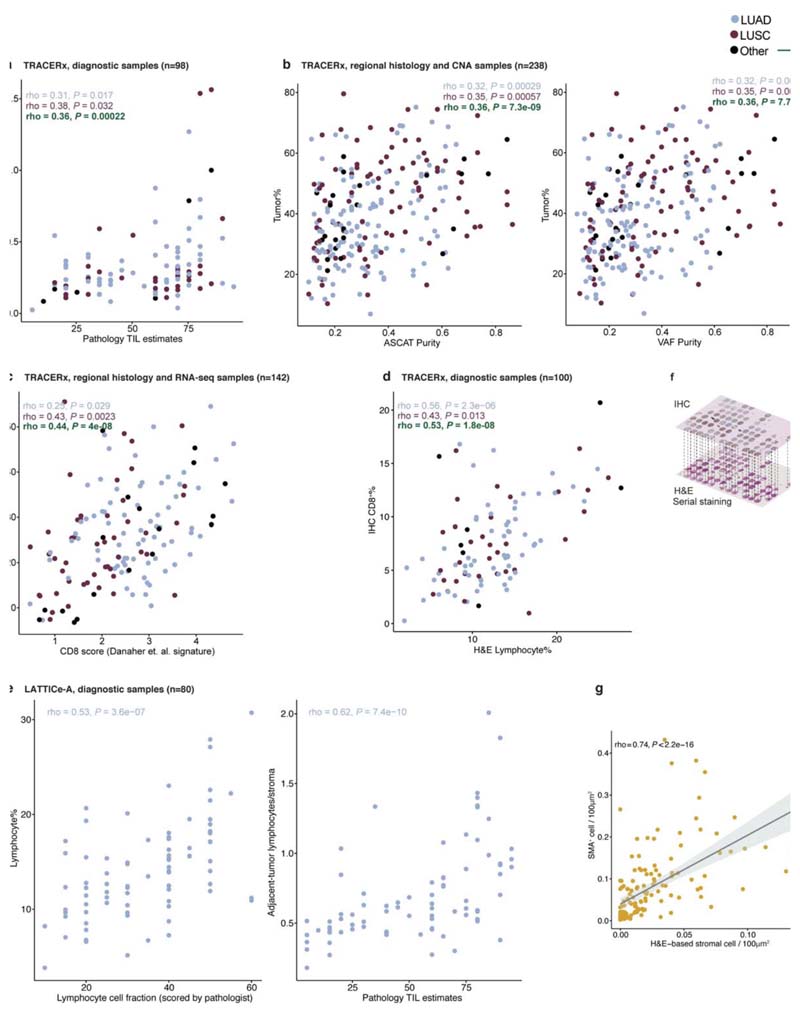
This pipeline for H&E analysis exhibited high accuracy and consistency compared with five orthogonal data types within TRACERx, including DNA-seq, RNA-seq, IHC, 5,951 single-cell annotations by pathologists (balanced accuracy, as an average of specificity and sensitivity = 0.932), and pathology tumor-infiltrating lymphocyte (TIL) estimates following the guidelines developed by the International Immuno-Oncology Biomarker Working Group⁷ (Extended Data Fig. 2, Supplementary Table 2). The Leicester Archival Thoracic Tumor Investigatory Cohort⁸ (LATTICe-A, Extended Data Fig. 1c-d), a retrospective study of 970 resected LUAD patients that included H&E sections from all diagnostic tumor blocks with a median of four samples per tumor, was used for independent validation. The pipeline’s generalizability was supported using 5,082 pathologists’ single-cell annotations (balanced accuracy = 0.913), and virtual integration of IHC and H&E images generated from the same slides (Fig. 1e-h, Extended Data Fig. 2e-g, Supplementary Table 3). Using this unbiased scalable approach, immune infiltration was quantified as the percentage of all cells that were lymphocytes in each H&E image.

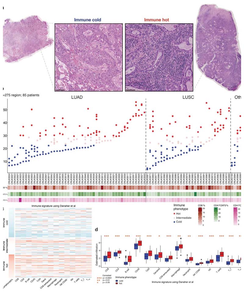
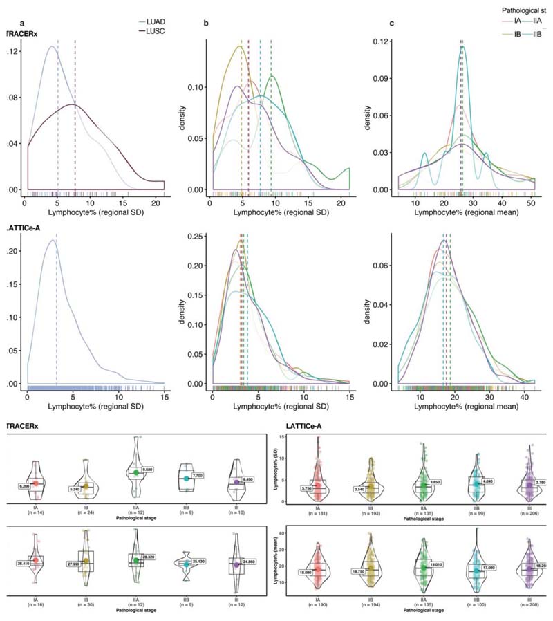
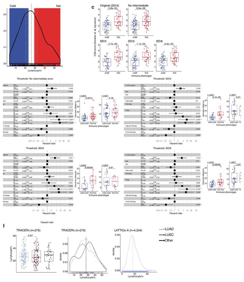
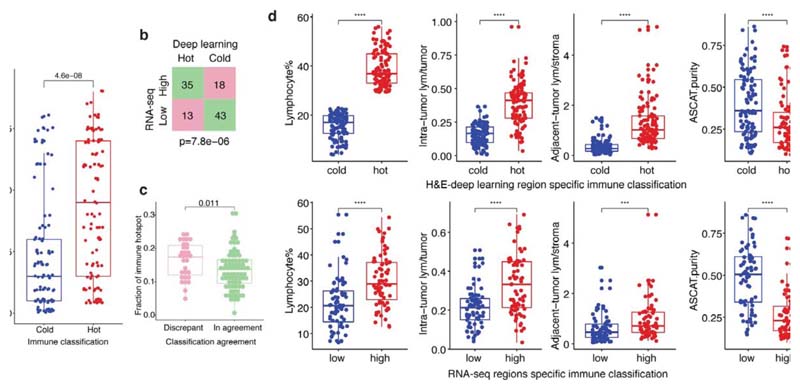
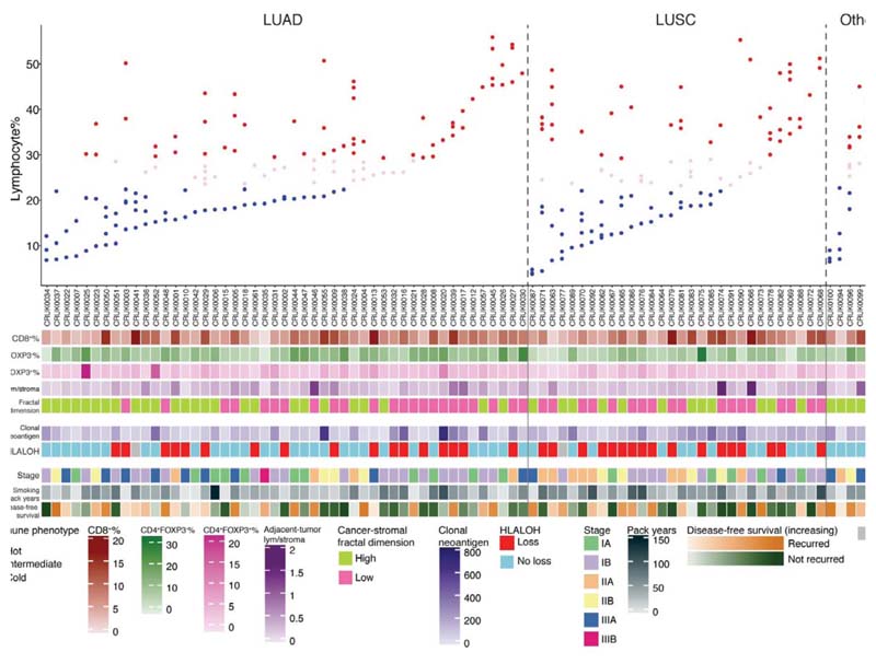
High geospatial immune variability between tumor regions within the same patients was revealed (Fig. 2a-b), which did not reflect associations with pathological stage (Extended Data Fig. 3). To differentiate highly from poorly immune infiltrated tumor regions, regions containing a lymphocyte percentage greater than a quarter standard deviation above the median lymphocyte percentage were classified as immune hot, and regions containing a lymphocyte percentage below a quarter standard deviation of the median were classified as immune cold. The remaining 20% were classified as intermediate (Fig. 2b). Subsequent results were tested on four more classification schemes based on the standard deviation to ensure that results derived from this classification were not contingent upon choice of thresholds used (Extended Data Fig. 4). Significant difference in pathology TIL estimates was observed between immune hot and cold regions (R = 4.6x10^-8, Extended Data Fig. 5a). Significantly higher levels of RNA-seq estimated immune infiltrate¹, particularly for immune activation subsets, were consistently observed in immune hot compared to cold regions, supporting the validity of histology-based immune classification (Fig. 2c-d). We next directly compared our immune hot and cold regional classification (excluding intermediate regions) against RNA-seq-based¹ classifications ( = 109 regions with histology and RNA-seq data). 78 out of 109 regions were in agreement (Fisher’s exact test for overlap: R = 7.8x10^-6, Extended Data Fig. 5b). Regions with discrepant classification ( = 31) had significantly higher spatial heterogeneity of lymphocyte distribution compared to regions concordant between the two methods (R = 0.01, Extended Data Fig. 5c), suggesting spatial intratumor heterogeneity could contribute towards the discrepancy, since the different data types were derived from adjacent sections of the same tumor blocks.

Figure 2. Geospatial heterogeneity of lymphocytic infiltration in the TRACERx cohort.

a. Representative examples of immune hot and immune cold multi-region H&E samples, scale bars represent 100μm. b. Each column represents a tumor, grouped by their histologic subtype (the “Other” group consists of adenosquamous carcinoma, large cell neuroendocrine carcinoma, pleomorphic carcinoma, and sarcomatoid carcinoma of pleomorphic type arising from adenocarcinoma). Tumor regions (illustrated as dots) were assigned to immune hot, immune cold, and intermediate phenotypes based on percentage of lymphocytes in all cells following H&E-based deep learning analysis. CD8⁺/CD4⁺FOXP3/CD4⁺FOXP3⁺ percentages based on automated analysis of the IHC diagnostic samples are also shown. c. A heatmap showing gene expression patterns of 14 immune cell populations across tumor regions, each row represents a tumor region (= 142). The three clusters correspond to the proposed immune regional classification as shown in b. d. Significant enrichment of all immune cell populations in hot regions, as compared to cold regions, particularly for the immune activating cell subsets, including cytotoxic, B-cell, and natural killer cells (= 109 regions; 52 patients). A two-sided, nonparametric, unpaired, Wilcoxon signed-rank test was used for each box plot, all R-values were corrected for multiple comparisons. Thick horizontal lines indicate the median value; outliers are indicated by the extreme points; the first and third quantiles are represented by the box edges; and vertical lines indicate the error range.

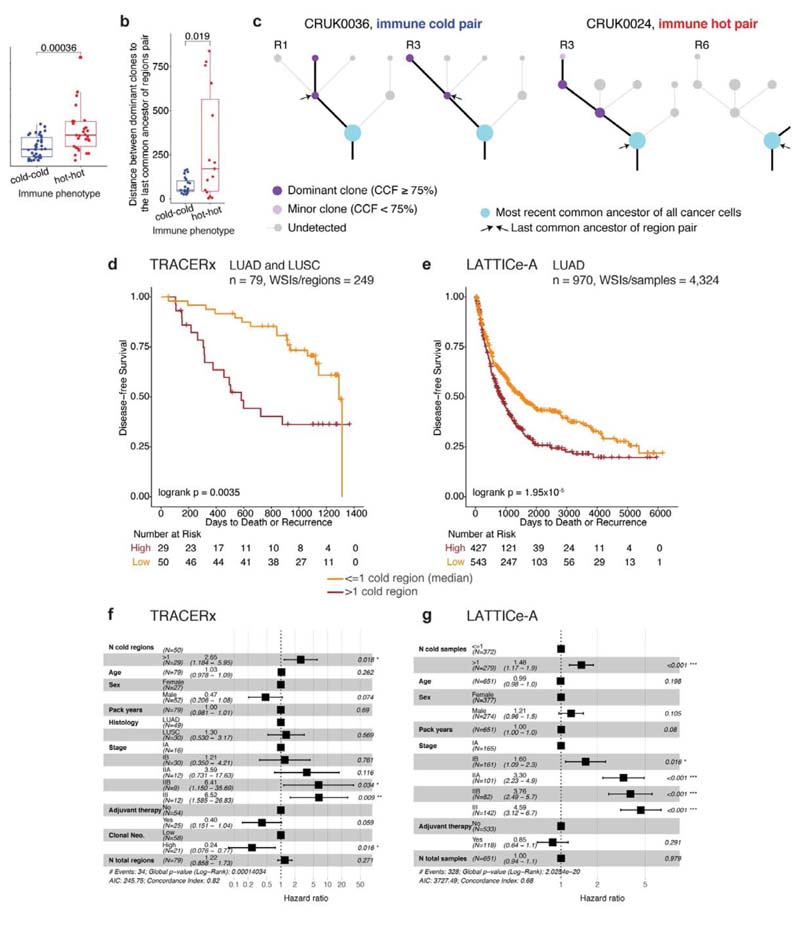
Ecological selection pressures drive genetic divergence^9,10. To determine if cancer genetic divergence differs according to immune context, we calculated the genomic distance as the Euclidean distance of subclonal mutations for each pair of tumor regions with the same immune phenotype in a patient. We observed significantly lower genomic distance, indicating more shared subclonal mutations, for pairs of immune cold regions than for pairs of immune hot regions in LUAD (Fig. 3a, Extended Data Fig.4b, R < 0.005 for all immune classification schemes), but not in LUSC (Extended Data Fig. 6a). In LUAD but not LUSC, analysis of immune phenotypes mapped onto the phylogenetic trees⁶ revealed that dominant clones (cancer cell fraction ≥ 75%, see Methods) in pairs of cold regions were more closely related on the phylogenetic tree, compared to dominant clones in pairs of immune hot regions (Fig. 3b). Moreover, dominant clones in hot regions almost always diversified at the most recent common ancestor of the tree (13/15, 87%, Fig. 3c), in contrast no such preference was observed in immune cold regions (11/23, 48%).

Figure 3. Evolution of immune escape, and survival analysis in TRACERx and LATTICe-A.

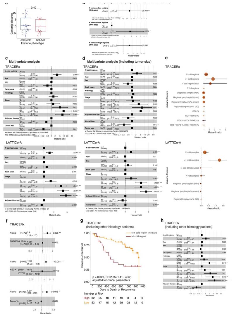
a. A box plot showing the difference in genomic distances for pairs of immune hot or immune cold regions within the same patients in LUAD (= 66 pairs), b. A box plot showing the difference in mutational distance between the dominant subclones in pairs of immune hot or immune cold regions via their last common ancestor in LUAD (= 23 immune cold pairs; 15 immune hot pairs). This distance was calculated by taking the furthest dominant clone (cancer cell fraction (CCF) ≥ 75%) from the trunk, and it remained significant when the dominant clone closest to the most recent common ancestor of each tree was considered (R = 0.02). c. Illustrative examples of tumor phylogenetic trees for a pair of immune hot and immune cold regions. Dominant subclones were labelled and their last common ancestor (annotated with arrows) was then identified. Minor (CCF < 75%) or undetected clones were neglected in this analysis. d,e. Kaplan-Meier curves illustrating the difference in disease-free survival according to the number of immune cold regions, dichotomized by the median value, in TRACERx (d) (LUAD and LUSC, = 79 patients, 249 regions) and LATTICe-A (e) (LUAD, = 970 patients, 4,324 samples). The same deep learning histology analysis and immune regional classification developed for TRACERx were applied directly to LATTICe-A. WSI: whole-section image, f. Forest plots showing multivariate Cox regression analyses in TRACERx (= 79 patients; LUAD and LUSC). Clonal neoantigens were dichotomized using the upper quartile, determined individually for LUAD and LUSC tumors¹. g. Forest plots showing multivariate Cox regression analyses in LATTICe-A (= 651 LUAD patients with complete stage and smoking pack years data). For the patient subset with complete stage data but missing pack years information, the test remained significant (= 827, R < 0.001, HR = 1.4[1.1-1.9]). For statistical comparisons among groups, a two-sided, non-parametric, unpaired, Wilcoxon signed-rank test was used, unless stated otherwise.

We investigated the impact of immune context on disease-free survival. Tumors with high number of immune cold regions were at significantly increased risk of relapse that was independent of the total number of regions sampled, tumor size and stage in both histology types in TRACERx (Fig. 3d-e, Extended Data Fig. 6c-h). This association with disease-free survival was also significant using the number of immune low regions as estimated by RNAseq¹ in 64 TRACERx tumors with available RNA-seq data (R = 0.002, Extended Data Fig. 6b). Following the genomic findings in LUAD, we sought to validate this in 970 LUAD patients in the multi-sample LATTICe-A cohort, confirming the prognostic value of immune cold sample count, that was also independent of the number of samples per patient, tumor size and stage (Fig. 3f-g, Extended Data Fig. 6c-e). In both cohorts, the number of immune cold samples per patient correlated with relapse, more significantly than any other immune feature generated using deep learning, including the average and variability of lymphocyte percentage per tumor, number of immune hot regions, proportion of immune cold regions to the number of regions sampled, as well as CD8⁺ cell percentage or CD8⁺ to CD4⁺FOXP3⁺ ratio in TRACERx diagnostic slides (Extended Data Fig. 6e).

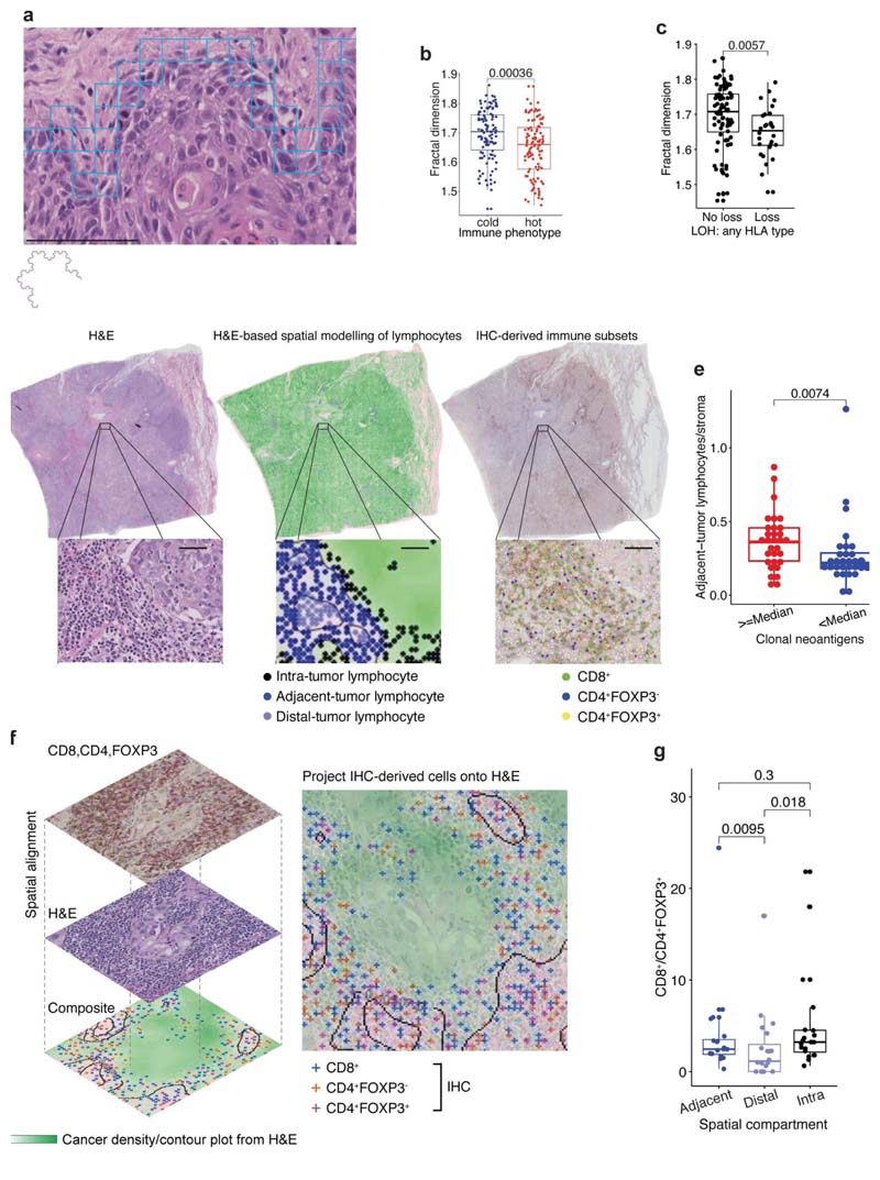
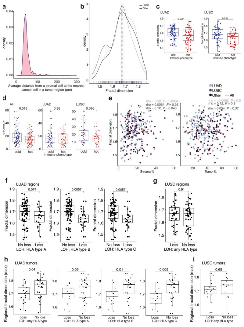
Studies have revealed immunosuppressive fibroblast subsets localizing to the boundary of tumor nests possibly contribute to T cell exclusion^11–13. Therefore, we hypothesized that increased cancer-stroma physical contact may reflect stroma-modulated inhibition of antitumor immune responses^14–17. To measure the physical contact between cancer and stromal cells (the majority being fibroblasts) identified by image analysis, we developed a spatial measure, using fractal dimension to quantify the geographical irregularity and complexity of the cancer-stromal cell interface (Methods, Fig. 4a, Extended Data Fig. 7a,b,e). Within the same tissue space, higher fractal dimension of cancer-stromal cell interface suggests increased geometric irregularity and more extensive physical contact between tumor and stromal cells than samples with a smooth interface. For both histology types, fractal dimension was significantly higher in immune cold regions compared to immune hot regions (Fig. 4b, Extended Data Fig. 7c). Moreover, the difference in fractal dimension between immune cold and hot regions was more significant compared to the difference in stromal cell percentage (both histology types combined: R = 0.00036, effectsize 0.49 for fractal dimension versus R = 0.018, effect size 0.38 for stromal cell percentage, Extended Data Fig. 7d), suggesting the importance ofstromal cell geographical location rather than their quantity. This supports the hypothesis that the stroma-based inhibition of immune infiltration¹⁷ may result from a specific topological pattern in the form of cancer-stroma engagement.

Figure 4. Association of spatial histology with genetic alterations relevant to immune surveillance.

a. An illustrative example of fractal dimension calculated by the box-counting algorithm to quantify the geospatial complexity of the cancer cell-stromal cell interface. By examining boxes of decreasing sizes that contain both cancer and stromal cells, the box counting algorithm quantifies the rate at which the geometrical details of cancer-stromal interface develop at increasingly fine scales. Blue box illustrates the smallest box of 20μm by 20μm in size. Scale bar represent 100μm. An example of a fractal structure displaying geometrical self-similarity is shown below the panel, b. A box plot to illustrate the significant difference in fractal dimension between all TRACERx immune hot and cold regions (= 219). c. A box plot showing a significant difference in fractal dimension between LUAD tumor regions (= 116) harboring an LOH event for class 1 HLA of any type versus regions that do not, adjusted for multiple comparisons with the remaining HLA type-specific tests (see Extended Data Fig. 7f). d. Illustration of the adjacent-tumor lymphocyte/stroma ratio inferred by spatial modeling of cancer cell density (contours) and lymphocyte classification into spatial compartments. Cell classification in IHC sample of the same block was shown for comparison. Scale bars represent 50μm. e. A box plot showing the difference in the adjacent-tumor lymphocyte/stroma ratio between high (≥ median) and low (< median) clonal neoantigens for all LUAD patients in TRACERx (= 61). f. Illustration of image registration to spatially align serial sections of H&E and IHC and generate a virtual composite map of T cell subset in the context of cancer/stroma density. T cell subsets classified in the IHC were projected onto the cancer density map inferred from H&E, so that they can be classified into adjacent-tumor, intra-tumor, and distal-tumor compartments, g. A box plot showing significantly higher ratio of CD8⁺ to CD4⁺FOXP3⁺ cells in adjacent-tumor and intratumor lymphocytes compared with distal-tumor lymphocytes in registered LUAD image tiles (= 20 image tiles, using paired Wilcoxon test). For statistical comparisons among groups, a two-sided, non-parametric, unpaired, Wilcoxon signed-rank test was used, unless stated otherwise.

To understand the associations of stromal-mediated immunosuppression in the context of the genetic mechanisms of immune evasion, we related fractal dimension to dysfunction in antigen presentation through loss of heterozygosity at the human leukocyte antigen locus (HLA LOH), which has been identified as a potent immune escape mechanism^1,18. A significantly higher fractal dimension was found in LUAD tumor regions with intact HLA alleles compared with regions harboring HLA LOH (Fig. 4c, Extended Data Fig. 7f). This was observed at the tumor level (see Methods for definition), independent of clonal neoantigen burden (R = 0.04, multivariate regression, Extended Data Fig. 7h), but was not observed in LUSC (Extended Data Fig. 7g, i).

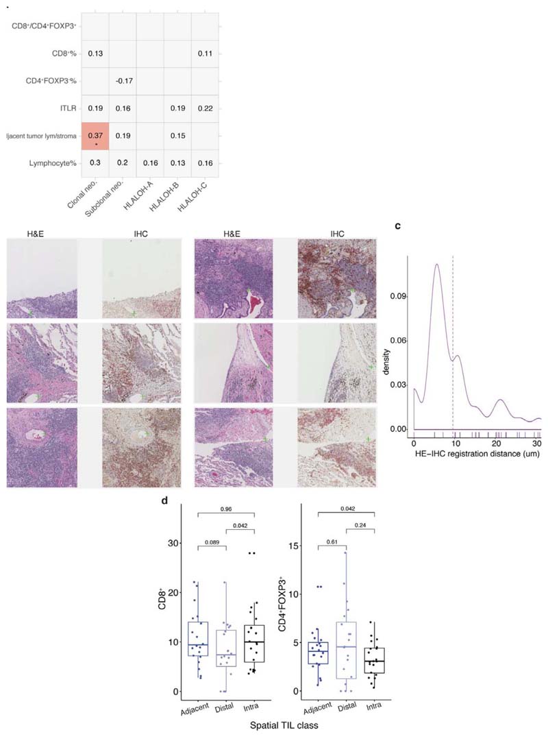
Although clonal neoantigens have been associated with a cytotoxic immune response¹⁹, the spatial distribution of lymphocytes in relation to clonal neoantigens remained unclear. To provide sufficient spatial context for analysis of cell distribution, whole-section TRACERx diagnostic H&E images, typically 10x larger than the regional samples, were used. To test the relationship between lymphocyte spatial distribution and clonal neoantigens, we leveraged an established method for lymphocyte spatial modeling²⁰. Each lymphocyte was classified into three distinct spatial compartments: intra-tumor, adjacent-to-tumor or distaltumor, based on unsupervised modeling of cancer-lymphocyte proximity (Fig. 4d). In LUAD, but not LUSC, clonal neoantigens¹⁹ were found to be associated with a specific immune spatial score to approximate pathology TIL estimates⁷, defined as the ratio of adjacenttumor lymphocytes to stromal cells in the diagnostic H&E samples (R = 0.0074, high clonal neoantigen defined as above median in LUAD, Fig. 4e; correlation as continuous variables Rho = 0.37, R = 0.035 after multiple testing correction, Extended Data Fig. 8a). By contrast, subclonal neoantigen burden did not correlate with any immune score (Extended Data Fig. 8a), supporting the notion that clonal but not subclonal neoantigens is associated with infiltration of cytotoxic T cells¹⁹ adjacent to tumor nests.

To determine if there was an enrichment of a specific lymphocyte subpopulation within the adjacent-tumor compartment in LUAD, we spatially aligned IHC to H&E in 10 samples with the highest adjacent-tumor lymphocytes to stromal cell ratio, and projected IHC-derived T cell subsets onto H&E images, thereby creating virtual staining of cells in the H&E sections (Methods, Fig. 4f, Extended Data Fig. 8b-c). CD4⁺FOXP3^-, CD8⁺, and CD4⁺FOXP3⁺ cells classified in IHC were projected onto a density map of cancer cell distribution inferred from H&E, and were classified into adjacent-tumor, intra-tumor, and distal-tumor compartments. In this limited dataset, a significant increase of the effector-regulator balance defined by CD8⁺/CD4⁺FOXP3⁺ cell ratio was observed in adjacent-tumor stroma compared to the distal tumor compartment (Fig. 4g).

In summary, by training deep learning algorithms in diverse histology samples, we demonstrated that digital pathology can provide accurate tools for defining the ecological spatial context that may improve our understanding of cancer evolution and the immune response. In TRACERx and LATTICe-A cohorts, LUAD tumors with increased immune cold regions were at a significantly higher risk of cancer relapse, independent of total regions sampled and immune phenotypes of other regions. Thus, even within a tumor that has on average increased immune infiltration, if it contains regions classified as immune cold, prognosis appears to be associated with the number of cold regions. Analysis of cancer branched evolution within the ecological context of immune hot and cold regions revealed a difference in the evolution history of cancer subclones in these regions, possibly as a result of immunoediting. Based on this finding, we speculate that by identifying the subclone where immunoediting is likely to have occurred, new drivers of immune evasion may be elucidated.

Spatial histology data can extend our knowledge of the tumor microenvironment topological configuration in relation to genetic alterations relevant to immune surveillance, including HLA LOH and clonal neoantigens in LUAD (Extended Data Fig. 9). Increased cancerstromal engagement as measured by fractal dimension may signal physical constraints against T cell ingress. This is supported by previous studies in lung cancer showing restriction of CD8⁺ and CD4⁺ T cell motility in dense stromal extracellular matrix areas around tumor epithelial cell regions which prevent them from entering tumor islets¹³. Additionally, the association between specific spatial localization of lymphocytes in tumoradjacent stroma and clonal neoantigens further support exploration of the role of stromal cells in limiting tumor infiltration by T cells^14–17.

It will be imperative to validate our findings on a larger multi-region cohort of untreated NSCLC tumors. Differences in our findings pertaining to LUAD and LUSC may reflect differences in biology^21–23 and immune evasion mechanisms, including increased prevalence of antigen presentation dysfunction (HLA transcriptional repression and HLA LOH¹) in LUSC. Other limitations include the lack of detailed staining using multiplexing technologies^24–26 that could provide further insights into immune composition. However, with advanced deep learning developments and detailed tumor phylogenetic data, histology can be used to highlight fundamental immune contexture such as immune exclusion and its topological determinants. These data illuminate the clinical significance of immune cold regions that may reflect immune evading subclones, warranting further investigation into mechanisms that could contribute to the spatial variability of immune cells.

Methods

Tissues and digital images

The main cohort evaluated comes from the first 100 patients prospectively analyzed by the lung TRACERx study⁶ (Extended Data Fig. 1, Supplementary Tables 1, 4, https://clinicaltrials.gov/ct2/show/NCT01888601, approved by an independent Research Ethics Committee, 13/LO/1546). 62 were men and 38 were women, with a median age of 68. 61 were LUAD, 32 were LUSC and the remaining 7 had ‘other’ histology subtypes (including adenosquamous carcinoma, large cell carcinoma, large cell neuroendocrine carcinoma, pleomorphic carcinoma and pleomorphic carcinoma arising from adenocarcinoma).

The 85 case subcohort with regional histology consisted of 55 male and 30 female patients and of those 49 were LUAD, 32 were LUSC and 6 were ‘other’ types. 10 of these patients had a single region while the rest ranged between 2-8 regions (= 275 total regional histology samples). Snap-frozen regional samples were processed to FFPE blocks after dissecting fresh-frozen tissues for DNA-seq and RNA-seq analyses. Tissue microarrays (TMAs) were created containing 133x2mm regional tissue cores from 75 patients in 7 blocks.

In addition to the regional samples, full-sized diagnostic blocks were obtained for all 100 cases precisely mirroring the Jamal-Hanjani et al. 2017 prospective 100 patient cohort⁶. 4μm thick sections were cut and subjected to H&E staining and multiplex IHC for CD8/CD4/FOXP3: anti-CD8 (type: Rabbit Monoclonal, clone: SP239, cat. no.: abl78089, source: Abeam Pic, Cambridge, UK, used at 1:100); anti-CD4 (type: Rabbit Monoclonal, clone: SP35, cat. no.: ab213215, source: Abeam Pic, Cambridge, UK, used at 1:50); antiFOXP3 (type: Mouse, clone: 236A/E7, source: kind gift from Dr G Roncador, CNIO, Madrid, Spain, used at: 1:100). All regional and diagnostic slides were scanned using NanoZoomer S210 digital slide scanner (C13239-01) and NanoZoomer digital pathology system version 3.1.7 (Hamamatsu, Japan) at 40x (228 nm/pixel resolution).

The external validation cohort was obtained from the Leicester Archival Thoracic Tumor Investigatory Cohort – Adenocarcinoma (LATTICe-A) study⁸, a continuous retrospective series of resected primary LUAD tumors from a single surgical center between years 1998 to 2014 (Extended Data Fig. 1, Supplementary Table 5). It consists of 4,324 whole-tumor diagnostic blocks from 970 LUAD patients (ranging from 1 to 16 blocks per case with a median of 4). 455 were men and 515 were women with a median age of 69. Most clinical data (age, sex, adjuvant therapy status and time to recurrence or death) were available for all patients, with complete pathological stage for 827 and smoking history for 651. All archival slides containing tumor material were used in order to capture the full diversity of each lesion. Slides were dearchived and scanned using a Hamamatsu NanoZoomer XR at 40x (226 nm/pixel resolution) yielding 15 TB of image data. Images containing incidental lymph node tissue were excluded to avoid confounding immune infiltration analysis. For the biological validation assay, a subset of 49 paraffin blocks from 49 patients was obtained from the same study, and from these a validation TMA was prepared, containing a single 1mm core from each case. The work was ethically approved by an NHS research ethics committee (ref. 14/EM/1159). This study complies with the STROBE guidelines.

The deep learning pipeline for cell detection and classification

The deep learning pipeline consists of three parts. First, the pipeline segments tissue regions utilizing multi-resolution input/output image features (Micro-Net²⁷). It was designed to capture global tissue context and learn weak features that could be important for identifying tissue boundary, but are often not achieved by other machine learning methods such as thresholding of the grey-scale image, active contours, watershed segmentation or Support Vector Machine-based training on local binary pattern features²⁷. Tissue segmentation removes background noise and artefacts and subsequently allows for more computationally efficient cell detection and accurate classification. Secondly, a cell detection model modified from SCCNN²⁸ predicts for each pixel the probability that it belongs to the center of a nucleus within tissue regions identified by Micro-Net. Nuclei are detected from the probability map obtained from the deep network. Lastly, a cell classification framework utilizes a neighboring ensemble predictor classifier coupled with SCCNN to classify each cell by type.

For tissue segmentation, each whole slide image was reduced to 1.25x resolution and segmented for tissue regions using Micro-Net-5 1 2²⁷ architecture. This architecture visualizes the image at multiple resolutions, captures context information by connecting intermediate deep layers and adds bypass connections to max-pooling to maintain weak features (Fig. 1b). 10 whole slide images were used to train the tissue segmentation network using MicroNet. The segmented images from the network were inspected visually and quantitatively (Supplementary Table 6, Supplementary Figures 1-20) to evaluate performance using an independent set of images.

The SCCNN adds two layers to conventional deep learning architecture for cell detection within the segmented tissue. SC1 estimates the location and probability of each pixel belonging to the center of a cell, and these probabilities are then mapped by SC2 to the image. A customized implementation of SCCNN was coded in Python (version 3.5) using TensorFlow²⁹ library (version 1.3) which makes it computationally more efficient compared to the original MATLAB implementation²⁸. To process an image of size 1000×1000 pixels, the Python implementation takes 4.8 seconds for nucleus detection compared to 41.0 seconds using the original implementation²⁸, excluding preprocessing which remained the same in both implementations (using MATLAB (version 2018b)). In addition, through empirical experimentation, we optimized the patch size to 31x31 instead of 27x27 in the original implementation for increased cell detection accuracy. To generate nuclear locations from the SC2 probability map, peak detection was applied where thresholds for intensity and minimum grouping distance were also optimized to 0.15 and 12 pixels through experimentation using validation data.

For cell classification, a neighboring ensemble predictor was used. This predictor utilizes SCCNN to classify cells in neighboring locations to the detected center of the cell. In our implementation, the ensemble classifier required votes from SCCNN classification of nine different neighborhood locations near to the center of the cell compared to five votes in original implementation. Through experimentation, the patch size was optimized to 51x51 for classification instead of 27x27 as originally proposed. This permitted incorporation of greater tissue spatial context while maintaining the accuracy of classifying small cells.

Altogether, this pipeline enabled the spatial mapping of four cell types from H&E images: cancer (malignant epithelial) cells, lymphocytes (including plasma cells), noninflammatory stromal cells (fibroblasts and endothelial cells), and an “other” cell type that included nonidentifiable cells, less abundant cells such as macrophages and chondrocytes, and ‘normal’ pneumocytes and bronchial epithelial cells.

Training the deep learning pipeline

To improve neural network generalizability and to avoid overfitting for cell detection and classification, we trained and tested our pipeline on a variety of sample types, including diagnostic (= 100), regional (= 275) and 133 cores corresponding to 75 TRACERx patients from TMA slides (63 patients had two cores and 12 patients had a single core). Both cell detection and classification were trained based on single-cell annotations from pathologists. Two thoracic pathologists annotated 26,960 cells on 53 whole slide images (3 TMAs, 35 regional slides and 15 diagnostic slides) to incorporate morphological variations in appearance of various cell types and stain variability. Several hundred examples of each cell class were marked on 76 cores selected at random from TMA images. In total, 4,056, 5,310, 15,007, 2,587 annotations were collected for stromal cells, lymphocytes, cancer cells and “other” cell types, respectively. These whole slide images were divided into small tile images of size 2000×2000 pixels (each pixel = 0.5μm), which were then divided into three sample sets maintaining the class distribution of cells. These included: 13 diagnostic, 58 regional and 134 TMA tile images for training; 4 diagnostic, 21 regional and 72 TMA tile images for validation; and 3 diagnostic, 22 regional and 61 TMA tile images for testing. As a result, the annotations were divided between the three groups; 2/3 for training, 1/6 for validation and 1/6 for testing. The training set included annotations for 2,147 stromal cells, 3,183 lymphocytes, 10,103 cancer and 1,357 other cell types. The validation set had annotations for 473 stromal cells, 825 lymphocytes, 2,562 tumor and 359 other cell types. Breakdown for the test set is provided in Supplementary Table 2.

For IHC cell classification, we used a pretrained SCCNN network on samples stained for CD4/CD8/FOXP3. The training set consisted of 1,657 CD4⁺FOXP3^-, 3,187 CD8⁺, 1,001 CD4⁺FOXP3⁺, and 3,488 other (negative) cells. The trained network was tested on 5,028 cell annotations collected on 6 lung diagnostic whole slide images, including 251 CD4⁺FOXP3^-, 406 CD8⁺, 123 CD4⁺FOXP3⁺ and 4,248 other cells to test the ability of the algorithm in correctly detecting and classifying negative cells. See Supplementary Table 7 for the total number of identified cells in the H&E diagnostic, H&E multi-region and IHC diagnostic datasets.

Validation of the H&E deep learning pipeline with orthogonal data types

The algorithms’ performance in detecting and classifying single cells in H&E were first evaluated against the test set of 5951 cells. Individual class accuracy statistics were calculated using the R function ‘confusionMatrix’ from the R package ‘caret’.

Pathology TIL estimates were scored following the international guidelines developed by the International Immuno-Oncology Biomarker Working Group⁷. Briefly, by inspection of H&E slide of a given tumor region, the fraction of the stromal area infiltrated by TILs was assessed.

For regional samples, tumor cellularity, estimated as the computed percentage cancer cells was correlated with tumor purity estimated by ASCAT based on DNA-seq copy number and VAF purity (both available from Jamal-Hanjani et al.⁶, = 239 regional tumor samples). The RNA-seq-based CD8⁺ T cell signature (available from Rosenthal et al.¹, computed using the Danaher et al. method³⁰) was correlated with the deep learning based lymphocyte percentage for 142 regional tumor samples. For diagnostic samples, deep learning-based lymphocyte percentage from H&E was correlated with deep learning-based CD8⁺ cell percentage from IHC (= 100 diagnostic samples, Extended Data Fig. 2a-d).

Discordance rate between RNA-seq based¹ and histology/deep learning-based immune hot and cold regional classification was calculated by cross-tabulation of immune hot and cold (from histology) versus high and low (from RNA-seq), disregarding any regions without one of these two types of data. The RNA-seq method used 15 immune cell signatures presenting different T- and B-cell subsets, as well as neutrophils, macrophages, mast and dendritic cells, to classify tumor regions into high and low categories. A Fisher’s exact test was used to compute the overlap between the two immune classifications. Distributions of multiple immune scores (lymphocyte percentage, intra-tumor lymphocytes and adjacent-tumor lymphocytes/stroma) as well as ASCAT tumor purity were compared between hot versus cold (deep learning) and high versus low (RNA-seq) classifications (Extended Data Fig. 5).

Validation of the deep learning pipeline with the independent LATTICe-A cohort

The external validity of the proposed deep learning pipeline was performed on 100 randomly selected patients from the LATTICe-A cohort⁸. This validation ensures that the trained cell detection and cell classification models from the TRACERx tumor blocks are generalizable to a distinct dataset which is processed, stained and scanned in another center (the LATTICe-A study, University of Leicester).

All 100 whole-tumor H&E sections were processed using the same TRACERx trained model. The validation was then performed using two data types. First, a pathologist provided 5,082 single-cell annotations following the same protocol for TRACERx in 20 randomly selected LATTICe-A sections. The breakdown for single-cell annotations was 1,997 stromal cells, 787 lymphocyte cells, 1,839 cancer cells and 459 other cells (see Supplementary Table 3). Second, two independent pathologists jointly scored the remaining 80 sections for overall fraction of lymphocytic infiltration and pathology TIL estimates⁷. These manual scores were correlated with the deep learning-based lymphocyte percentage and adjacent-tumor lymphocytes/total stroma (Extended Data Fig. 2e).

Validation of the deep learning pipeline with biological assays

A new biological validation method was developed to overcome the challenge of obtaining large quantities of cell-specific validation data (Fig. 1f-h, Extended Data Fig. 2f-g). 48 cores were available for the TTF1-H&E image pairs, 38 for the CD45-H&E pairs, and 33 for the SMA-H&E pairs. Stains were performed using a Ventana BenchMark ULTRA instrument (H&E, TTF-1) or a Dako Link 48 (CD-45, SMA). Digital images were acquired using a Hamamatsu Nanozoomer slide scanner. First, H&E staining was performed using a Leica Infinity kit, and a digital image was collected. The slide was subsequently de-coverslipped, the H&E stain removed by acid alcohol washing, and then an immunohistochemical stain with haematoxylin counterstain was applied using a standard diagnostic antigen retrieval and antibody protocol. A second digital image was acquired after mounting and coverslipping. Through experimentation, no difference in the staining was observed when the procedure was reversed.

TTF-1 (type: Novocastra Liquid Mouse Monoclonal antibody thyroid transcription factor 1, clone: SPT24, cat. no.: NCL-L-TTF-1, source: Leica biosystems, Germany, used at 1:100) was selected as the cancer cell marker in these LUAD samples because it is the most robust and widely used immunohistochemical marker of LUAD cells³¹. It is very specific, both in that only epithelial cells are stained in the lung, and in that very few tumors of non-lung or thyroid origin are stained³². The sensitivity of the antibody clone used (SPT24) is also high, staining >75% of tumor cells in 76% of LUAD tumors in one published series³³. However, as this implies, there are many tumors in which tumor cell staining is incomplete (i.e. <100%). Therefore, only cores showing near-universal TTF-l-positivity of tumor cells were used for validation, in order to provide the best possible ‘gold standard’ comparator for the deep learning algorithm. The same procedure was followed for pairs of H&E-CD45 (anti-human CD45, type: Mouse Monoclonal, clone: 2B11 + PD7/26, cat. no.: M0701, source: Agilent DAKO, USA, used at 1:200) and H&E-SMA (myofibroblast marker, type: Mouse Monoclonal antibody Smooth Muscle Actin (1A4), cat. no.: 760-2833, source: Roche, Switzerland, a ready to use antibody) to biologically validate the accuracy of single cell classification.

In total, 64,976 TTF1⁺ cells, 26,284 CD45⁺ cells and 46,343 SMA⁺ cells were detected from the IHC images, denoting the advantage of this method in acquiring large amount of validation data at single-cell resolution. The correlation measured (Fig. 1f-h, Extended Data Fig. 2g) was that between the fraction of classified cells in the H&E versus fraction of positively stained IHC cells per 100μm².

Immune phenotype classification

To classify tumor regions into different immune phenotypes, we assigned each region to an immune hot, cold or intermediate category based on lymphocyte percentage. The dependency of our subsequently results on thresholds chosen for this classification scheme was tested after applying perturbations to the thresholds used. Four new classification schemes were tested: no intermediate zone (i.e. using median lymphocyte percentage for separating hot and cold regions), regions with lymphocyte percentage greater than standard deviation/2 above/below the median lymphocyte percentage classified as immune hot/cold,, and similarly for standard deviation/3 and standard deviation/6 (Extended Data Fig. 4a-b). For every new classification, we repeated the multivariate survival analysis to confirm the significance of the number of immune cold regions in predicting disease-free survival as well as the genomic distance test for pairs of immune hot versus immune cold regions in LUAD patients (Extended Data Fig. 4b). In addition, the CD8⁺ RNA-seq signature was used to test the difference in CD8⁺ levels between immune hot and immune cold phenotypes across all classification schemes (Extended Data Fig. 4c).

Genomic distance measure

Genomic distance was calculated as described previously¹, by taking the Euclidean distance of the mutations present for every pair of immune hot and immune cold regions from the same patient. All mutations present in a region from a tumor were turned into a binary matrix of which the rows were mutations and columns were the tumor regions. From this matrix, the pairwise distance was determined.

Distance between dominant clones to the last common ancestor of region pair

Deep learning-based immune phenotypes were integrated with the TRACERx phylogenetics data⁶. Dominant clones (using the upper quartile of cancer cell fraction, ≥ 75%) were labelled for all tumor regions’ trees which had an available H&E sample in LUAD patients (= 76 regions, 15 immune hot pairs and 23 immune cold pairs). For every pair of immune hot ≥ cold regions within a tumor, the distance between the dominant clones (as measured by branch length, i.e. number of mutations) via their last common ancestor was computed. The recently shared ancestry clone between the two dominant clones was labelled as the ‘last common ancestor of region pair’ (annotated with arrows in Fig 3.c). To ensure this analysis was not dependent on a certain cancer cell fraction threshold, multiple thresholds (CCF ≥ 80%, 85%) were placed while repeating the same analysis. Next, by identifying the last common ancestral subclone for pairs of the same phenotype, each pair was categorized into one of two diversification patterns: ‘diversifying at the most recent common ancestor (MRCA) of the tree’ or ‘diversifying at a descendant subclone of the MRCA of the tree’. The latter category included a pattern exclusive to immune cold pairs, where the two regions shared the same dominant subclone that was the direct descendant of the MRCA of the tree.

Tumor spatial modelling

H&E and IHC cell abundance scores (e.g. lymphocyte percentage, CD8⁺ percentage) were computed as the percentage of a cell type in the total sample cell count. Stromal TILs were identified using spatial modelling^20,34,35, where lymphocytes were classified (using unsupervised clustering) into intra-tumor lymphocytes, adjacent-tumor lymphocytes and distal-tumor lymphocytes based on their spatial proximity to epithelial cell nests in H&Es. The immune hotspot score was calculated using the Getis-Ord algorithm as previously described³⁶. To capture the emergence of complex morphological patterns that dictate cancer-stromal cell spatial contact preserved over varying spatial scales, a fractal dimension calculation (Minkowski-Bouligand dimension) was performed using the boxcounting algorithm³⁷. This algorithm calculates the number of boxes of a certain size needed to cover a geometric pattern. We modified a MATLAB-based algorithm³⁸ to include both spatial information of cancer and stromal cells, as opposed to its conventional use on one variable (i.e. pixel information of an image). The analysis was carried out on spatial maps generated using coordinates of classified stromal and cancer cells, while utilizing the tissue segmented image (as a boundary mask) to exclude all empty tissue areas. Choices of box size were informed by the distribution of minimum and maximum Euclidean distance for each stromal cell to its nearest cancer cell in all 275 tumor regions (Extended Data Fig. 7a). The mean minimum distance was 21.43μm. We limited the upper box size at 300μm, which is just above a previously proposed cell-cell communication distance of 250μm³⁹ but designed to be more inclusive. For statistical tests where fractal dimension was represented at tumor level, the maximum regional score was used.

H&E-IHC spatial alignment/immune subset projection

For a H&E diagnostic slide, we determined the number of intra-tumor lymphocytes, adjacent-tumor lymphocytes and distal-tumor lymphocytes (n_I, n_A, n_D) based on spatial modelling of the H&Es. After spatial alignment of IHC and projecting IHC-derived cells onto the H&E, the number of CD8⁺ cells that were also intra-tumor lymphocytes was determined (n^CD8 _ITL), and similarly for other cell types. As a result, intra-tumor lymphocytes were deconvolved by n_I = n^CD8 _I, + n^CD4 _I, + n^FOXP3, + n^other _I. Two-sided paired Wilcox was used to test the difference in the percentage of CD8⁺ cells among intra-tumor lymphocytes, adjacent-tumor lymphocytes and distal-tumor lymphocytes (n^CD8 _ATL, n^CD8 _DTL, n^CD8 _ITL). The same test was performed for CD4⁺FOXP3^- and CD4⁺FOXP3⁺ cells.

The 10 LUAD patients with the highest adjacent-tumor lymphocytes to stromal cell ratio were selected for this immune subset spatial projection. All samples had above median CD8⁺%. One sample was excluded due to poor HE-IHC alignment quality and the subsequent analysis was performed on the remaining nine samples. The quality of alignment was evaluated by manually identifying 238 visible landmarks and placed on corresponding positions in H&E and IHC tiles (total number of tiles = 249, maximum landmarks per tile = 5), as shown in Extended Data Fig. 8b. These marked points were used to compute the Euclidean distance (difference in, coordinates) between them to obtain a quantitative measurement ofalignment accuracy. The average distance between matching landmarks was 9.57μm, whereas the maximum distance between the H&E and CD4/CD8/FOXP3 sections was 16μm.

Survival analysis and other statistical methods

Survival tests were conducted using Kaplan-Meier estimator (‘ggsurvplo’ R function from the ‘survminer’ and ‘survival’ R packages) as well as Cox model (‘coxph’ R function and displayed using ‘ggfores’ R function). Forest plots show the hazard ratio in the x-axis; each variable’s hazard ratio is plotted and annotated with a 95% confidence interval. The clinical parameters included in the multivariate model were age, sex, smoking pack years, histology (whether LUAD, LUSC or otherwise), tumor stage, adjuvant therapy (whether received or not). Because of its prognostic importance in TRACERx, the upper quartile of clonal neoantigens in each histology cohort was also incorporated in the multivariate model. The range of available disease-free survival data was 34-1364 days (median = 915 days) in TRACERx, and 1-6139 days (median = 684 days) in LATTICe-A. All hazard ratios were computed on all time points (i.e. the whole survival curve, not at a specific time point). Correlation tests used Spearman’s method and were generated using the function ‘ggscatter’ from the ‘ggpubr’ R package. All correlation plots show the Rho (ρ) coefficient and the significance R-value. For statistical comparisons among groups, a two-sided, non-parametric, unpaired, Wilcoxon signed-rank test was used, unless stated otherwise. All box plots were generated using the function ‘ggboxplo’ from the ‘ggpubr’ R package (all data points are plotted with the ‘jitter’ option, the median value is indicated by a thick horizontal line; minimum and maximum values are indicated by the extreme points; the first and third quantiles are represented by the box edges; and vertical lines indicate the error range) or the function ‘ggbetweenstats’ from the ‘ggstatplo’ R package for more than two groups. Tests for concordance between two data classes were analyzed using a Fisher’s exact test. All statistical tests were two-sided, a R value of less than .05 was considered statistically significant. To adjust R-values for multiple comparisons, the Benjamini & Hochberg method was used. To measure effect size, Cohen’s d method was used. All statistical analyses were conducted in R (version 3.5.1).

Extended Data

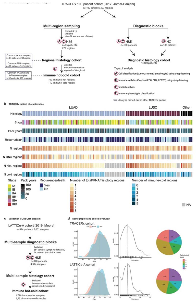
Extended Data Fig. 1. CONSORT diagrams for TRACERx 100 and LATTICe-A histology cohorts and patient characteristics.

a. TRACERx CONSORT diagram to illustrate sample collection and analysis of regional and diagnostic histology samples, as well as the overlap with RNA and DNA studies. b. TRACERx patient characteristics for the histology cohort. c. LATTICe-A CONSORT diagram (= 970 LUAD patients). Legends for ‘type of the analysis’ correspond to panel a. d. Demographics and clinical patient characteristics for TRACERx (top three panels) and LATTICe-A (bottom three panels) showing the distribution of age (colored by sex), distribution of smoking pack years and the proportion of patients in each pathological stage. Horizontal lines indicate the median value.

Extended Data Fig. 2. Validation of the automated single-cell classification for H&E.

a. A scatter plot showing the correlation between H&E-based adjacent-tumor lymphocytes/stromal and pathology TIL estimates in diagnostic samples (= 98 diagnostic slides/patients). b. Scatter plots showing the correlations between H&E-based tumor cellularity estimate and ASCAT/VAF purity scores (= 238 regions; 83 patients). c. A scatter plot showing the correlation between H&E-based estimate of lymphocyte percentage among all cells and RNA-seq-based CD8⁺ signature using the Danaher et al. method³⁰ (= 142 regions; 56 patients). d. A scatter plot showing the correlation between H&E-based estimate of lymphocyte percentage among all cells and CD8⁺ cell percentage in IHC in the diagnostic samples (= 100 diagnostic slide/patients). e. Scatter plots showing the correlation between H&E-based lymphocyte percentage versus pathological scores of overall lymphocytic cell fraction, and adjacent-tumor lymphocytes/stromal versus pathology TIL estimates in an external cohort (LATTICe-A, = 80 diagnostic slides/patients). f. Illustrative example to show the spatial alignment of TTFl/CD45/SMA-stained IHC and H&E images obtained using sequential staining on the same tissue microarray section for biological validation, g. A scatter plot showing the correlation between stromal cell percentage determined by H&E and SMA⁺ cell percentage per LUAD image tiles of size 100μm² (= 144). The experiment was conducted once using one TMA (= 33 cores/patients). The shading indicates 95% confidence interval.

Extended Data Fig. 3. Distribution of regional lymphocytic infiltration according to pathological stage.

All available patients’ data have been used in this figure except for the standard deviation tests excluding patients with a single tumor region. Patients without pathological staging information from the LATTICe-A cohort were also removed. a, b, c, top row: TRACERx and bottom row: LATTICe-A. Horizontal lines indicate the median value. a. Distribution of the standard deviation of regional lymphocyte percentage for LUAD and LUSC patients in TRACERx (= 69), and LUAD in LATTICe-A (= 814). b. Distribution of the standard deviation of regional lymphocyte percentage across pathological stages (= 69 for TRACERx, 814 for LATTICe-A). c. Distribution of regional mean of lymphocyte percentage across stages (= 79 for TRACERx, 827 for LATTICe-A). d. No significant difference among stages with respect to standard deviation (= 69 for TRACERx, 814 for LATTICe-A) or mean (= 79 for TRACERx, 827 for LATTICe-A) of regional lymphocytic infiltration. Left panel, TRACERx and right panel, LATTICe-A. Correction for multiple testing was applied in d, for each cohort individually. A two-sided, non-parametric, unpaired, Wilcoxon signed-rank test was used; each dot represents a patient; the mean value is annotated with a large dot; the median value is represented by a thick horizontal line; minimum and maximum values are indicated by the extreme points; the first and third quantiles are represented by the box edges; and the violin shape shows the data distribution as a kernel density estimation.

Extended Data Fig. 4. Validation of immune phenotype classification.

a. The proposed immune classification imposed on density plot showing distribution of lymphocyte percentage. The middle zone corresponds to the intermediate phenotype, red zone for immune hot and blue zone for immune cold. Black dash line shows the median. This classification was validated after applying small perturbations to the thresholds to reclassify regional immune phenotypes, illustrated as grey dash lines: no intermediate zone (i.e. hard median for separating hot and cold), standard deviation (SD)/2 above and below the median, SD/3 and SD/6. b. Forest plots to show repeated multivariate Cox regression tests for the number of immune cold regions using these new classifications (= 79 patients), after accounting for stage, total number of samples, upper quartile of clonal neoantigens determined for LUAD and LUSC individually, and other clinical parameters. Box plots showing difference in genomic distance for pairs of hot regions compared with pairs of cold regions for LUAD and LUSC separately (LUAD: = 45 hot pairs, 45 cold pairs for no intermediate zone; = 19 hot, 25 cold for SD/2; = 25 hot, 33 cold for SD/3; = 32 hot, 41 cold for SD/6. LUSC: = 32 hot pairs, 54 cold pairs for no intermediate zone; = 19 hot, 27 cold for SD/2; = 19 hot, 37 cold for SD/3; = 27 hot, 41 cold for SD/6.). c. Box plots showing significant difference in CD8⁺ RNA-seq signature using the Danaher method between regions of hot and cold phenotype across all classification schemes (= 219 for SD/4; 275 for no intermediate zone; 173 for SD/2; 204 for SD/3; 237 for SD/6). d. Distribution and difference of lymphocytic infiltration for LUAD versus LUSC regions in TRACERx (= 275 regions; 85 patients) as well as distribution for LUAD in LATTICe-A (= 4,324 samples; 970 patients). Horizontal lines in the distribution plots indicate mean values. For statistical comparisons among groups, a two-sided, non-parametric, unpaired, Wilcoxon signed-rank test was used, unless stated otherwise.

Extended Data Fig. 5. Concordance between histology deep learning and RNA-seq immune classification.

a. A box plot showing the difference in pathology TIL estimates between immune hot and immune cold regions (= 219). Pathology TIL estimates score fraction of stroma containing TILs, whereas immune classification was defined based on the percentage of lymphocytes in all cells within a slide, b. A confusion matrix to compare RNA-seq and deep learning histology immune classifications (discarding immune intermediate regions, = 109 regions (57 LUAD, 37 LUSC, 15 other histology subtypes); 52 patients). The p-value was generated using a two-sided Fisher’s exact test for overlap. c. A box plot showing the difference in the fraction of immune hotspots³⁶ in regions where the two classifications are in agreement (= 78; labeled as ‘In agreement’) against the discrepant regions (= 31, labeled as ‘Discrepant’). Each dot represents a region, the median value is indicated by a thick horizontal line; minimum and maximum values are indicated by the extreme points; and the first and third quantiles are represented by the box edges. d. Box plots to support the overall consistency between H&E-deep learning and RNA-seq methods by comparing different immune scores as well as ASCAT tumor purity between immune hot/high and cold/low tumor regions (all R-values < 0.0001). Top row, H&E-deep learning immune classification (= 219; except the ASCAT purity box plot = 186 regions), bottom row, RNAseq derived immune classification (= 142; except the ASCAT purity box plot, = 141 regions). For statistical comparisons among groups, a two-sided, non-parametric, unpaired, Wilcoxon signed-rank test was used, unless stated otherwise.

Extended Data Fig. 6. Genomic and survival analysis of tumor regions according to immune phenotypes.

a. A box plot showing the difference in genomic distances for pairs of immune hot versus immune cold regions within the same LUSC patients (= 59 pairs). A two-sided, non-parametric, unpaired, Wilcoxon signed-rank test was used. b. Forest plots to show the univariate prognostic value for the number of immune low regions (both as continuous and dichotomized at the median (≤1 versus >1)), or the number of immune high regions, using the immune classification generated by RNA-seq-based infiltrating immune cell populations¹ in 64 TRACERx tumors (41 LUAD, 16 LUSC and 7 other histology subtypes). c. Forest plots showing multivariate Cox regression analyses in both TRACERx (= 79 patients; LUAD and LUSC combined) and LATTICe-A (= 651 LUAD patients representing a subset with complete stage and smoking pack years data) with the number of immune cold regions dichotomized at the median (≤1 versus >1). This remains significant when the number of immune cold regions was replaced as a continuous variable, in the same multivariate model, (R = 0.019 in TRACERx and < 0.001 in LATTICe-A, for the number of immune cold regions). Clonal neoantigens were dichotomized using the upper quartile, determined individually for LUAD and LUSC tumors¹. d. The same test in c when tumor size (in mm) was also controlled in the multivariate model in LATTICe-A. This test also remained significant for a bigger group of patients with complete stage data, but missing pack years information (= 815, R < 0.001, HR = 1.4[1.1-1.8]). e. Forest plots to compare the prognostic value of regional immune scores as well as diagnostic H&E and IHC scores for relapse-free survival in TRACERx (= 79 patients, LUAD and LUSC combined). Wherever possible, these immune features were tested in LATTICe-A (= 970 patients). To compare the prognostic value of the number of immune cold region with other immune features, LATTICe-A comparisons were conducted in Cox multivariate regression models to include every immune feature after correcting for the number of immune cold regions in the same model. Each variable’s HR is plotted with a 95% confidence interval; all R-values were adjusted for multiple testing; and the size of the circles denotes–log₁₀(R). For the sake of visualization, a minor adjustment was made to the HR for the number of cold regions/total number of regions in LATTICe-A from 0.88[0.57-1.3] to 0.99[0.97-1.3], SD: standard deviation, used for measuring variability of lymphocyte percentage among samples within a tumor, f. Forest plots using Cox multivariate regression analysis showing that the prognostic value of the number of immune cold regions was independent of: 1) genetic measure, subclonal copy number alteration (obtained from ⁶); 2) tumor cellularity from DNA-seq-based ASCAT purity, 3) tumor cellularity measured by deep learning-based cancer cell percentage, g. Kaplan Meier curves to illustrate the difference in relapse-free survival for TRACERx patients including other histology types (= 85; representing all TRACERx patients in the multiregion histology cohort) with high and low number of immune cold regions, dichotomized by its median value. Log-rank R = 0.0017. h. Forest plot using Cox regression for the multivariate survival analysis for the number of immune cold regions in TRACERx including patients with other histology subtypes (= 85).

Extended Data Fig. 7. Fractal dimension and relationships with stromal cells.

a. Distribution of the average minimum Euclidean distance between a stromal cell to its neighboring cancer cell. For every stromal cell in a tumor region slide, the minimum distance to nearest cancer cell was computed. This distance was then averaged for all identified stromal cells in every region to plot the distribution (= 275 regions; 85 patients). b. Distribution of the fractal dimension of the cancer-stroma cell interface for histology types in the TRACERx cohort (= 275 regions; 85 patients). c. Box plots to show the difference in fractal dimension between immune hot and cold regions in TRACERx LUAD (= 113) and LUSC (= 84). d. Box plots showing the difference in stromal cell percentage between immune hot and cold regions in all (= 219), LUAD (= 113), and LUSC (= 84). e. Scatter plots showing the correlation between fractal dimension and percentage of cells that are stromal or cancer in all tumor regions (= 275 regions; 85 patients). This shows that fractal dimension was independent of tumor cell composition, with only a weak correlation with stromal cell percentage and no correlation with tumor cellularity. f. Box plots showing the difference in fractal dimension between LUAD tumor regions harboring an LOH event for HLA type A (= 106), type B (= 113), type C (= 108) versus regions that do not, adjusted for multiple comparisons with the corresponding test in Fig. 4c. g. The same test in f repeated for LUSC tumor regions (= 87) for HLA of any type. h. Box plots showing the difference in tumor-level fractal dimension using the maximum value of regional measures between LUAD tumors (= 48) harboring a single LOH event for any HLA type, HLA type A, type B and type C versus tumors that do not, independent of predicted clonal neoantigens. Each p-value was generated using a multiple regression linear model and was also adjusted for multiple testing correction. i. The same test in h repeated for LUSC tumors (= 29) for HLA of any type. For statistical comparisons among groups, a two-sided, non-parametric, unpaired, Wilcoxon signed-rank test was used, unless stated otherwise.

Extended Data Fig. 8. Relationship of immune subsets and spatial TILs in LUAD.

a. Spearman’s correlations between immune scores in diagnostic slides and genetic measures including predicted neoantigens and HLALOH in LUAD patients (= 46). ITLR: intra-tumor lymphocytes to total tumor cell ratio. Only significant correlations after multiple testing are highlighted (rho = 0.37, R = 0.035). b. Examples of registered H&E and IHC tiles. The green cross denotes a manually placed landmark repeated 238 times on pairs of H&E-IHC image tiles. The Euclidean distance (difference in, coordinates) was computed between the two landmarks which was then c. shown as a distribution to represent the accuracy of the registration (= 249 total H&E-IHC image tiles, maximum five landmarks per a pair of tiles). The average distance between matching landmarks was 9.57μm and the distribution is within the expected range of maximum distance between four serial sections (16μm). d. Box plots to illustrate the difference in percentage of immune cell subsets among adjacent, intra and distal-tumor lymphocytes (= 20 image tiles), a non-parametric, paired Wilcoxon test was used.

Extended Data Fig. 9. Summary of immune and genomics features in NSCLC.

An extended heatmap showing all immune variables described in TRACERx across all patients (= 275 regions; 85 patients), along with genetic measures and clinical parameters. Each column represents a tumor, grouped by their histologic subtype. Tumor regions (illustrated as dots) were assigned to immune hot, immune cold and intermediate phenotypes based on percentage of lymphocytes in all cells following H&E-based deep learning analysis. Cancerstromal fractal dimension, defined using the maximum fractal dimension in regions of a patient, using the median as cut-off to determine high and low groups.

Reporting summary.

Further information on research design is available in the Nature Research Reporting Summary linked to this paper.

Data availability

The digital pathology images from the TRACERx study generated or analysed during this study are not publicly available and restrictions apply to its use. A test subset of such digital pathology images are available through the Cancer Research UK & University College London Cancer Trials Centre (ctc.tracerx@ucl.ac.uk) for non-commercial research purposes and access will be granted upon review of a project proposal that will be evaluated by a TRACERx data access committee and entering into an appropriate data access agreement, subject to any applicable ethical approvals. Digital pathology images for LATTICe-A samples with expert pathologist’s annotations used for validation are available: https://github.com/qalid7/compath. Request for data access for the remaining LATTICe-A samples can be submitted to J.L.Q.

Code availability

The deep learning pipeline for digital pathology image analysis is available for noncommercial research purposes: https://github.com/qalid7/compath. All code used for statistical analyses of image data was developed in R version (3.5.1) and is available: https://github.com/qalid7/tx100_compath.

References

- 1.Rosenthal R, et al. Neoantigen-directed immune escape in lung cancer evolution. Nature. 2019;1 doi: 10.1038/s41586-019-1032-7. [DOI] [PMC free article] [PubMed] [Google Scholar]
- 2.Morris LGT, Chan TA. Lung Cancer Evolution: What’s Immunity Got to Do with It? Cancer Cell. 2019;35:711–713. doi: 10.1016/j.ccell.2019.04.009. [DOI] [PubMed] [Google Scholar]
- 3.Morris LGT, et al. Pan-cancer analysis of intratumor heterogeneity as a prognostic determinant of survival. Oncotarget. 2016;7:10051–10063. doi: 10.18632/oncotarget.7067. [DOI] [PMC free article] [PubMed] [Google Scholar]
- 4.Milo I, et al. The immune system profoundly restricts intratumor genetic heterogeneity. Scì Immunol. 2018;3 doi: 10.1126/sciimmunol.aat1435. [DOI] [PubMed] [Google Scholar]
- 5.Jia Q, et al. Local mutational diversity drives intratumoral immune heterogeneity in non-small cell lung cancer. Nat Commun. 2018;9 doi: 10.1038/s41467-018-07767-w. [DOI] [PMC free article] [PubMed] [Google Scholar]
- 6.Jamal-Hanjani M, et al. Tracking the Evolution of Non-Small-Cell Lung Cancer. N Engl J Med. 2017;376:2109–2121. doi: 10.1056/NEJMoa1616288. [DOI] [PubMed] [Google Scholar]
- 7.Hendry S, et al. Assessing Tumor-Infiltrating Lymphocytes in Solid Tumors. Adv ANat Pathol. 2017;24:311–335. doi: 10.1097/PAP.0000000000000161. [DOI] [PMC free article] [PubMed] [Google Scholar]
- 8.Moore DA, et al. In situ growth in early lung adenocarcinoma may represent precursor growth or invasive clone outgrowth—a clinically relevant distinction. Mod Pathol. 2019;1 doi: 10.1038/s41379-019-0257-1. [DOI] [PubMed] [Google Scholar]
- 9.Whittaker KA, Rynearson TA. Evidence for environmental and ecological selection in a microbe with no geographic limits to gene flow. Proc Natl Acad Scì U S A. 2017;114:2651–2656. doi: 10.1073/pnas.1612346114. [DOI] [PMC free article] [PubMed] [Google Scholar]
- 10.Shafer ABA, Wolf JBW. Widespread evidence for incipient ecological speciation: A meta-analysis of isolation-by-ecology. Ecology Letters. 2013;16:940–950. doi: 10.1111/ele.12120. [DOI] [PubMed] [Google Scholar]
- 11.Costa A, et al. Fibroblast Heterogeneity and Immunosuppressive Environment in Human Breast Cancer. Cancer Cell. 2018;33:463–479.:e10. doi: 10.1016/j.ccell.2018.01.011. [DOI] [PubMed] [Google Scholar]
- 12.Öhlund D, et al. Distinct populations of inflammatory fibroblasts and myofibroblasts in pancreatic cancer. J Exp Med. 2017;214:579–596. doi: 10.1084/jem.20162024. [DOI] [PMC free article] [PubMed] [Google Scholar]
- 13.Salmon H, et al. Matrix architecture defines the preferential localization and migration of T cells into the stroma of human lung tumors. J Clin Invest. 2012;122:899–910. doi: 10.1172/JCI45817. [DOI] [PMC free article] [PubMed] [Google Scholar]
- 14.Thomas DA, Massague J. TGF-ß directly targets cytotoxic T cell functions during tumor evasion of immune surveillance. Cancer Cell. 2005;8:369–380. doi: 10.1016/j.ccr.2005.10.012. [DOI] [PubMed] [Google Scholar]
- 15.Joyce JA, Fearon DT. T cell exclusion, immune privilege, and the tumor microenvironment. Science (80-) 2015;348:74–80. doi: 10.1126/science.aaa6204. [DOI] [PubMed] [Google Scholar]
- 16.Sorokin L. The impact of the extracellular matrix on inflammation. Nat Rev Immunol. 2010;10:712–723. doi: 10.1038/nri2852. [DOI] [PubMed] [Google Scholar]
- 17.Chen DS, Mellman I. Elements ofcancer immunity and the cancer-immune set point. Nature. 2017;541:321–330. doi: 10.1038/nature21349. [DOI] [PubMed] [Google Scholar]
- 18.McGranahan N, et al. Allele-Specific HLA Loss and Immune Escape in Lung Cancer Evolution. Cell. 2017;171:1259–1271.:e11. doi: 10.1016/j.cell.2017.10.001. [DOI] [PMC free article] [PubMed] [Google Scholar]
- 19.McGranahan N, et al. Clonal neoantigens elicit T cell immunoreactivity and sensitivity to immune checkpoint blockade. Science (80-) 2016;351 doi: 10.1126/science.aaf1490. [DOI] [PMC free article] [PubMed] [Google Scholar]
- 20.Yuan Y. Modelling the spatial heterogeneity and molecular correlates of lymphocytic infiltration in triple-negative breast cancer. J R Soc Interface. 2015;12:20141153. doi: 10.1098/rsif.2014.1153. [DOI] [PMC free article] [PubMed] [Google Scholar]
- 21.Thomas A, Liu SV, Subramaniam DS, Giaccone G. Refining the treatment of NSCLC according to histological and molecular subtypes. Nat Rev Clin Oncol. 2015;12:511–526. doi: 10.1038/nrclinonc.2015.90. [DOI] [PubMed] [Google Scholar]
- 22.Hammerman PS, et al. Comprehensive genomic characterization of squamous cell lung cancers. Nature. 2012;489:519–525. doi: 10.1038/nature11404. [DOI] [PMC free article] [PubMed] [Google Scholar]
- 23.Collisson EA, et al. Comprehensive molecular profiling of lung adenocarcinoma: The cancer genome atlas research network. Nature. 2014;511:543–550. doi: 10.1038/nature13385. [DOI] [PMC free article] [PubMed] [Google Scholar]
- 24.Keren L, et al. A Structured Tumor-Immune Microenvironment in Triple Negative Breast Cancer Revealed by Multiplexed Ion Beam Imaging. Cell. 2018;174:1373–1387.:e19. doi: 10.1016/j.cell.2018.08.039. [DOI] [PMC free article] [PubMed] [Google Scholar]
- 25.Giesen C, et al. Highly multiplexed imaging of tumor tissues with subcellular resolution by mass cytometry. Nat Methods. 2014;11:417–422. doi: 10.1038/nmeth.2869. [DOI] [PubMed] [Google Scholar]
- 26.Goltsev Y, et al. Deep Profiling of Mouse Splenic Architecture with CODEX Multiplexed Imaging. Cell. 2018;174:968–981.:e15. doi: 10.1016/j.cell.2018.07.010. [DOI] [PMC free article] [PubMed] [Google Scholar]
- 27.Raza SEA, et al. Micro-Net: A unified mode1 for segmentation of various objects in microscopy images. Med Image Anal. 2019;52:160–173. doi: 10.1016/j.media.2018.12.003. [DOI] [PubMed] [Google Scholar]
- 28.Sirinukunwattana K, et al. Locality Sensitive Deep Learning for Detection and Classification of Nuclei in Routine Colon Cancer Histology Images. IEEE Trans Med Imaging. 2016;35:1196–1206. doi: 10.1109/TMI.2016.2525803. [DOI] [PubMed] [Google Scholar]
- 29.Abadi M, et al. TensorFlow: Large-Scale Machine Learning on Heterogeneous Distributed Systems. 2016.
- 30.Danaher P, et al. Gene expression markers of Tumor Infiltrating Leukocytes. J Immunother Cancer. 2017;5:18. doi: 10.1186/s40425-017-0215-8. [DOI] [PMC free article] [PubMed] [Google Scholar]
- 31.Holzinger A, et al. Monoclonal Antibody to Thyroid Transcription Factor-1: Production, Characterization, and Usefulness in Tumor Diagnosis. Hybridoma. 1996;15:49–53. doi: 10.1089/hyb.1996.15.49. [DOI] [PubMed] [Google Scholar]
- 32.Matoso A, et al. Comparison of thyroid transcription factor-1 expression by 2 monoclonal antibodies in pulmonary and nonpulmonary primary tumors. Appl Immunohistochem Mol Morphol AIMM. 2010;18:142–9. doi: 10.1097/PAI.0b013e3181bdf4e7. [DOI] [PMC free article] [PubMed] [Google Scholar]
- 33.Pelosi G, et al. ΔNp63 (p4O) and Thyroid Transcription Factor-1 Immunoreactivity on Small Biopsies or Ce1lblocks for Typing Non-small Ce1l Lung Cancer: A Nove1 Two-Hit, Sparing-Material Approach. J Thorac Oncol. 2012;7:281–290. doi: 10.1097/JTO.0b013e31823815d3. [DOI] [PubMed] [Google Scholar]
- 34.Heindl A, et al. Re1evance of Spatial Heterogeneity of Immune Infiltration for Predicting Risk of Recurrence After Endocrine Therapy of ER+ Breast Cancer. JNCI J Natl Cancer Inst. 2018;110 doi: 10.1093/jnci/djx137. [DOI] [PMC free article] [PubMed] [Google Scholar]
- 35.Heindl A, et al. Microenvironmental niche divergence shapes BRCAl-dysregulated ovarian cancer morphological plasticity. Nat Commun. 2018;9:3917. doi: 10.1038/s41467-018-06130-3. [DOI] [PMC free article] [PubMed] [Google Scholar]
- 36.Nawaz S, Heindl A, Koe1ble K, Yuan Y. Beyond immune density: critical role of spatial heterogeneity in estrogen receptor-negative breast cancer. Mod Pathol. 2015;28:766–777. doi: 10.1038/modpathol.2015.37. [DOI] [PubMed] [Google Scholar]
- 37.Dubuc Quiniou, Roques-Carmes Tricot, Zucker Evaluating the fractal dimension of profiles. Phys Rev A, GeN Phys. 1989;39:1500–1512. doi: 10.1103/physreva.39.1500. [DOI] [PubMed] [Google Scholar]
- 38.MOISY F, JIMENEZ J. Geometry and clustering of intense structures in isotropic turbulence. J Fluid Meeh. 2004;513:111–133. [Google Scholar]
- 39.Francis K, Palsson BO. Effective interce1lular communication distances are determined by the re1ative time constants for cyto/chemokine secretion and diffusion. Proc Natl Acad Sci U S A. 1997;94:12258–62. doi: 10.1073/pnas.94.23.12258. [DOI] [PMC free article] [PubMed] [Google Scholar]
Associated Data
This section collects any data citations, data availability statements, or supplementary materials included in this article.
Supplementary Materials
Data Availability Statement