An open access mouse brain flatmap and upgraded rat and human brain flatmaps based on current reference atlases.

Abstract

Here we present a flatmap of the mouse central nervous system (brain) and substantially enhanced flatmaps of the rat and human brain. Also included are enhanced representations of nervous system white matter tracts, ganglia, and nerves, and an enhanced series of ten flatmaps showing different stages of rat brain development. The adult mouse and rat brain flatmaps provide layered diagrammatic representation of central nervous system divisions, according to their arrangement in corresponding reference atlases: Brain Maps 4.0 (BM4, rat) (Swanson, 2018), and the first version of the Allen Reference Atlas (mouse) (Dong, 2007). To facilitate comparative analysis, both flatmaps are scaled equally, and the divisional hierarchy of gray matter follows a topographic arrangement used in BM4. Also included with the mouse and rat brain flatmaps are cerebral cortex atlas level contours based on the reference atlases, and direct graphical and tabular comparison of regional parcellation. To encourage use of the brain flatmaps, they were designed and organized, with supporting reference tables, for ease-of-use and to be amenable to computational applications. We demonstrate how they can be adapted to represent novel parcellations resulting from experimental data, and we provide a proof-of-concept for how they could form the basis of a web-based graphical data viewer and analysis platform. The mouse, rat, and human brain flatmap vector graphics files (Adobe Reader/Acrobat viewable and Adobe Illustrator editable) and supporting tables are provided open access; they constitute a broadly applicable neuroscience toolbox resource for researchers seeking to map and perform comparative analysis of brain data.

Graphical Abstract

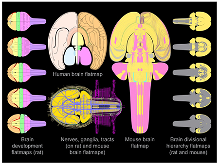
The illustration shows several flatmap representations of the mammalian brain, selected and modified from a collection of new and enhanced flatmap representations of the mouse, rat, and human brain. The human brain flatmap primarily details cortical regionalization. The rat and mouse brain flatmaps are based on current brain reference atlases, and they represent all depths of the divisional hierarchy of central nervous system gray matter represented therein. Also represented for rat and mouse are white matter tracts, ganglia, and nerves, and for the rat a series of flatmaps illustrating stages of brain development. The rat and mouse brain flatmaps are designed to facilitate comparative analysis between these species, and for adaptability to novel parcellation schemas and computational applications. We give examples of these uses, including a proof-of-concept workflow demonstrating how the flatmaps could be adapted to form the basis of a web-based graphical data viewer and analysis platform to represent a wide variety of brain data.

1. Introduction

Diagrammatic communication of knowledge is an ancient human practice, and a very useful aid to understanding complex structures such as the brain and nervous system. Diagrammatic representation of the complex three-dimensional (3-D) structure of the brain as a two-dimensional (2-D) map—a flatmap—is useful because it provides a relatively simple and effective way to summarize and compare brain data that is spatially localized (for examples see Hahn et al., 2019; Hahn & Swanson, 2015)—a quality that applies to all brain data but varies with respect to spatial resolution (granularity) (Swanson & Bota, 2010; Swanson & Lichtman, 2016).

As a starting point for the flatmaps for the adult mouse brain and the adult and developing rat brain presented here, we used previously created flatmaps for the developing and adult rat nervous system (Swanson, 2018) that were modelled on a flatmap representation of the topologically flat embryonic neural plate (Alvarez-Bolado & Swanson, 1996; Swanson, 1992). For embryonic stages occurring after neurulation begins and the neural plate develops into the neural tube, bilateral brain flatmap production is likened to making a dorsal cut through the roofplate lengthwise along the neural tube, then flattening each side along the straightened floorplate. Similarly, adult brain flatmap production is likened to making a dorsal midline cut lengthwise through the brain, then opening the left and right side as one would open a printed book, with the spine of the book at the ventral midline (Alvarez-Bolado & Swanson, 1996; Swanson, 1992, 2018). The human brain flatmap presented here primarily details cerebral cortex regionalization, and is modelled on an initial version (Swanson, 1995) created using an approach analogous to that used for the rat brain flatmap.

For the mouse and rat, in addition to flatmap representation of the brain, also included for both rodents is flatmap representation of the nerves, ganglia, and white matter tracts of the nervous system, based on their previous representation for the rat (Swanson, 2018). Therefore, collectively, the flatmap diagrams represent the mammalian nervous system, exemplified for the rat, through stages of development from embryo to adult. However, because the emphasis of the flatmaps presented here is the central nervous system (CNS), they are referred to simply as brain flatmaps. The brain flatmap versions presented here for mouse, rat, and human are as follows: adult mouse brain flatmap version 1.0 (MsBF1), adult rat brain flatmap version 5.0 (RtBF5), developing rat brain flatmaps version 2.0 (RtDevBF2), and human brain flatmap version 3.0 (HuBF3). The most recent previous versions of the rat (version 4.0 for adult, and 1.0 for development) and human (version 2.0) brain flatmaps were presented together in Brain Maps 4.0 (BM4) (Swanson, 2018), and were used as templates for the present versions; rat brain flatmap version 4.0 was also used as the template for MsBF1.

For the present rat and human brain flatmaps, nomenclature follows BM4. For the mouse brain flatmap, nomenclature follows the first version of the Allen Reference Atlas (ARAv1) (Dong, 2007) for gray matter regions and their subregions. As defined previously (Swanson & Bota, 2010), and elaborated in BM4, gray matter regions are “…recognizable volumes of gray matter that are distinguished by a unique set of neuron types with a unique spatial distribution…” and are considered to “…occupy the lowest basic level, roughly analogous to species in biological taxonomy…” (see Table C introduction in Supporting Information 8 in Swanson, 2018).

For ARAv1 gray matter divisions above the level of gray matter region (their parent divisions), the more recent BM4 nomenclature is applied. The rationale for this is three-fold. First, ARAv1 nomenclature was presented in a structure-function arrangement based on the arrangement in the third edition of Swanson’s Rat Brain Maps (BM3, the predecessor to BM4) (Swanson, 2004), whereas BM4 nomenclature is arranged strictly topographically, facilitating comparison with the vertebrate nervous system generally, and the human nervous system specifically (Swanson, 2015a). Second, all gray matter regions and their subdivisions described in ARAv1 assign to the topographically arranged and hierarchically organized parent divisions defined in BM4, and they do so quite easily because (with rare exception) ARAv1 parcellation and nomenclature is consistent with BM3 that (except for its different arrangement) is mostly consistent with BM4. Third, informed by recent efforts to codify neuroanatomical terminology into a unified taxonomy (Swanson, 2015a; Swanson & Bota, 2010), the internally consistent BM4 nomenclature serves as a foundational resource for a future pan-mammalian (and eventually pan-vertebrate) neuroanatomical nomenclature. Therefore, MsBF1 is aligned with a current systematic taxonomic approach to the organization of the mammalian nervous system (Swanson, 2018), supporting future inter-species comparative analysis.

A major upgrade included for RtBF5 is representation of all depths of brain divisions defined in BM4, including parent divisions, all gray matter regions, and their lowest level subdivisions—in BM4, and its earlier versions, these divisions were represented selectively on the flatmap. Similarly, all gray matter regions and their lowest level subdivisions described in ARAv1 are represented on MsBF1, along with all depths of parent divisions described in BM4. As we shall describe, the present rat and human brain flatmaps include several additional upgrades and enhancements, and these are applied similarly to the mouse brain flatmap. Apropos of these updates, a recent companion study to the present work is noteworthy (Swanson & Hahn, 2019), in which is presented an updated flatmap for the rat hippocampal formation, and a novel flatmap for the mouse hippocampal formation, including atlas level contours based on BM4 and ARAv1.

The design of the present brain flatmaps, including the organization of their constituent vector graphics layers, was guided by the goal of optimizing the visual display of information for ease of use and comparative analysis. To support this goal, the mouse and rat brain flatmaps, and accompanying comparison tables, together identify correspondences and differences between the underlying mouse (ARAv1) and rat (BM4) brain atlases. To demonstrate adaptability of the brain flatmaps to novel data, we provide two examples for MsBF1 using experimental data from our group: the first is a more granular parcellation of the caudoputamen based on the organization of input connections from the cerebral cortex (Hintiryan et al., 2016); the second is an alternative parcellation for the hippocampal formation based on a combination of gene expression and connectivity data (Bienkowski et al., 2018). In addition to these examples, using MsBF1 we also discuss and demonstrate how brain flatmaps could be used as the basis for a web-based brain flatmap data viewer and analysis tool.

2. Methods

The foundation of the brain flatmaps for the mouse and rat presented here are corresponding brain reference atlases for the mouse (ARAv1) (Dong, 2007) and rat (BM4) (Swanson, 2018) that include methodological details of atlas construction. Similarly, methodological details for the construction of the previous version of the adult rat brain flatmap in BM4 (Swanson, 2018), and its three predecessors (Swanson, 1992; Swanson, 1998; Swanson, 2004), are given in the earlier publications, and the essential basis for these (that applies to all the flatmaps) was described in the introduction. Methods are also previously described for the construction of earlier versions of the human brain flatmap (Swanson, 1995; Swanson, 2018), and rat brain developmental maps (Alvarez-Bolado & Swanson, 1996). The methods used here for brain flatmap construction follow the earlier methods and, as for previous brain flatmap versions, essentially involved the use of Adobe Illustrator (Ai) software to create the layered vector graphics files that comprise the flatmaps (consolidated as a single master file in Supporting Information 1, and as separate files in Supporting Information 2). Tutorials for Ai provided by Adobe are available freely online (https://helpx.adobe.com/illustrator/tutorials.html).

Description of the brain flatmap diagrams and supporting tables (that constitute the results) also describes their design implicitly, which is therefore integrated into the results, rather than repeated separately in the methods. The names and abbreviations of structures labeled on the brain flatmaps are defined in BM4 (Swanson, 2018) and ARAv1 (Dong, 2007); they are also available online for the mouse (http://help.brain-map.org/displav/mousebrain/Documentation). and for the rat (https://sites.google.com/view/the-neurome-project/brain-maps). The definitions of abbreviations for gray matter divisions are also included here in tabular form in Supporting Information 3. Abbreviations of structures relating example data for MsBF1 are defined in the corresponding publications (Bienkowski et al., 2018; Hintiryan et al., 2016; Zingg et al., 2018), and they are also included here in corresponding sections of the results and discussion.

3. Results

3.1. Rat brain flatmap version 5.0 (RtBF5)

3.1.1. Overview of brain flatmap upgrades

It is convenient to begin with a description of version 5.0 of the rat brain flatmap (RtBF5) because most of the design principles also apply to version 1.0 of the mouse brain flatmap (MsBF1), and in general to version 3.0 of the human brain flatmap (HuBF3), and to version 2.0 of the rat brain developmental flatmaps (RtDevBF2). All the flatmap diagrams were created in Ai software (version 24) and each is provided in two files: 1) in a consolidated master file (Supporting Information 1) containing all the flatmaps in Adobe’s portable document format (PDF), with layering preserved as in the original Ai file when opened in Ai; 2) in one of four individual PDF files (Supporting Information 2) created from the consolidated file for the four different flatmap categories: MsBF1, RtBF5, RtDevBF2, HuBF3. The individual PDF files follow the same general layer sequence and naming as the consolidated file, but several major nested sublayers are promoted to top-level layers. The layer nesting was modified to support customizable viewing by toggling display of the top-level Ai file layers when the PDF is opened with Adobe Reader (Adobe’s free PDF viewer software) or Adobe Acrobat (the commercial version of Adobe Reader)—a feature that may be useful for research or educational purposes (especially for users who do not have access to commercial Ai software).

Here RtBF5 is revised and enhanced substantially from version 4.0 in BM4. In general, the graphics have been streamlined for more consistent representation of similar structural properties, applied to the attributes of line art, text, and colors. An upgraded color-coding is applied to an overview of major parts of the CNS (Figure 1), that is also applied consistently here to the mouse, human, and rat brain developmental flatmaps. A major enhancement for RtBF5 is flatmap representation of all depths of the nested topographically arranged divisional hierarchy of gray matter of the rat CNS, as described in BM4 (see Table C in Supporting Information 8 in Swanson, 2018), (Figure 2, Supporting Information 3). Beginning with the nervous system division of CNS at the top of the hierarchy (depth 1), it is 12 levels deep, including up to 9 depths of division above the level of gray matter region (parent divisions), and 2 below (subregions). Accordingly, following BM4, for each side (left and right) of the CNS there are represented 143 parent divisions, 418 gray matter regions, and 122 subregions (Figure 2). In addition, cortical lamination is represented for gray matter regions of the cerebral and cerebellar cortices. The previous rat brain flatmap in BM4 represented most, but not all, gray matter regions, and partially represented subregions, and parent divisions; cerebral cortex layers were not represented on the BM4 flatmap. A limited previous update to the BM4 flatmap is noted that was applied for purposes of illustration to the hypothalamus only (a flatmap version number is not assigned to the restricted update) (Hahn et al., 2019).

Figure 1.

A color-coded flatmap representation of major divisions of the vertebrate central nervous system. The flatmap template shown is based on one created previously for the adult rat that was itself based on rat brain development fatemaps (see text for details). The same overview template is used here for rat and mouse brain flatmaps; an updated human brain flatmap overview follows the same color scheme (see Figure 8).

Figure 2.

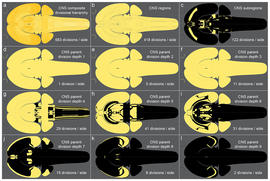
Flatmap representation of the nested divisional hierarchy of the rat central nervous system (CNS), following Brain Maps 4.0 (Swanson, 2018), and used here in RtBF5. The top left panel (a) shows the composite CNS divisional hierarchy, comprised of 143 parent divisions (above the level of gray matter region), 418 gray matter regions, and 122 subregions (for each side—left and right—of the CNS; excepting divisions that are cortical lamina). The tiles for each division are delineated, and semi-transparent to create an impression of the depth of nesting. Panels b-l represent the individual hierarchical divisions of the CNS: Panels b and c represent (respectively) gray matter regions, and subregions; panels d-l represent each of the 9 depths of CNS parent division. Yellow shading indicates the presence of a given division, whereas a black background indicates its absence. The two curved lines to the left of each panel represent the retina (a gray matter region division of the hypothalamus).

A list of the BM4 gray matter regions that were added to the flatmap for RtBF5 are given in Supporting Information 3; the annotated list also describes minor corrections and refinements to the BM4 flatmap that were applied to certain gray matter regions and subregions. In addition, to accommodate representation of all 418 gray matter regions in RtBF5, minor adjustments were made to the delineation of several division borders; refinements were also applied to the delineation of cerebral cortex divisions in conjunction with minor revisions to cerebral cortex atlas level contours (described in a later results section). A notable example is the olfactory bulb and neighboring regions of the cerebral cortex that were revised to improve alignment of cerebral cortex atlas level contours with a refined flatmap representation of the underlying gray matter regions. Nevertheless, because the changes are minor overall, and the same template scaling is used, data mapped to the previous version of the flatmap (or its predecessor that differs little) can be transferred and remapped to the current version with minimal adjustment.

3.1.2. Adobe illustrator file layering

Central to the design of RtBF5 is the arrangement and nesting of the Ai file layers. RtBF5 has 93 main layers to a depth of 5 nested levels. Version 2.0 of the flatmaps for rat brain development (RtDevBF2) has 116 main nested layers (to a depth of 5). Therefore, to a depth of 5 nested levels, the present rat brain flatmap Ai file versions for the adult rat (RtBF5), and developing rat (RtDevBF2), have a combined 209 main layers. To facilitate layer navigation and use of the Ai file, each of the Ai file layers is named concisely, and they are also color-coded using a simple system: the default layer indicator color for RtBF5 and RtDevBF2 layers is magenta; it is light red for sublayers containing text, light blue for line art sublayers, and bright green for tile (filled shape) sublayers. Accordingly, the different graphic elements of text, line art, and tiles are placed in separate color-coded layers.

Details of layer naming and color-coding for RtBF5 are provided in a separate Microsoft Excel spreadsheet (Excel) file (Supporting Information 4) that recapitulates the arrangement and color-coding of the main nested layers present in the Ai file and provides explanatory annotations for individual numbered layers. Supporting Information 4 also lists the nested color-coded layers used for MsBF1 (default layer color cyan) and HuBF5 (default layer color yellow). User-initiated filtering of nested layers is enabled to one or more selected depth (from a depth of 1 to 5). The consolidated brain flatmap file for mouse, rat, and human (Supporting Information 1) has a total of 353 main nested layers (93 for RtBF5; 116 for RtDevBF2; 120 for MsBF1; 24 for HuBF5). Additional subsidiary sublayers are also present in the Ai file that are not listed on the spreadsheet (Supporting Information 4) to avoid unnecessary repetition (and reduce spreadsheet length) because their contents are self-evident from their layer names and guided also by the name of the parent layer(s). For example, the RtBF5 layer named “Legend (color key)” is a sublayer to the layer named “Nerves, Ganglia, Tracts (rat)” and has 7 sublayers not listed on the spreadsheet that are named according to the part of the legend that they correspond to (for example, “CNS white matter tracts”). Another example is provided by the deepest nested sublayers of the layer named “CNS White Matter Tracts (179)” (row 138 in the Excel file Supporting Information 4): the name of each of the sublayers is the abbreviation of the corresponding white matter tract graphics represented therein. Also noteworthy is that the number in parenthesis (of row number 138) is the number of the white matter tracts (for one side of the brain)—totals are given similarly in parenthesis in the layer names of each major structural division.

3.1.3. Nerves, ganglia, and white matter tracts

Introduced for the rat brain flatmap in BM4 was a comprehensive representation of the nerves and ganglia of the peripheral nervous system (PNS), and CNS white matter tracts. In BM4 a two-color red/green color scheme was used to represent these structures (red for nerves and tracts, and primarily green for ganglia). However, the two-color scheme limits differentiation of structures belonging to different divisional groupings and prevents differentiation of closely juxtaposed nerves and tracts. These issues were ameliorated in BM4 by grouping structure abbreviation text with the corresponding structure graphic in the Ai file. The latter precedent is followed here, and to improve Ai file navigation the layer name for each ganglion, nerve, and tract is the abbreviation for the corresponding named structure. In addition, the abbreviation-named layers are listed alphabetically to help identify the location of structures of interest on the flatmap (an arrangement also applied to gray matter division layers). Furthermore, to improve visual structural differentiation, and to avoid a predominantly red/green color scheme that could also be problematic for individuals with the most common type of colorblindness, a more varied and contrasting color scheme is applied here. Additionally, lines representing autonomic and cranial nerves, and white matter tracts, are selectively semi-transparent and gradient-shaded longitudinally enabling visual differentiation of apposed parallel lines and conveying the impression of 3-D at higher zoom levels. Visual structural differentiation is also reinforced by abbreviation text style, with italics used for all nerves and tracts, and non-italicized text for ganglia. A further enhancement, that applies to the entire flatmap, is the introduction of an optional inner black- and outer dark gray background for customizable viewing in a light or dark mode (Figure 3).

Figure 3.

Graphical upgrades to the flatmap representation of the nerves and ganglia of the peripheral nervous system (PNS), and central nervous system (CNS) white matter tracts (tracts). As shown in (a), different divisional groupings are represented by contrasting colors, with a different shade of the same color used to both indicate and differentiate PNS nerves and ganglia belonging to the same divisions, as shown in the key below (a). The flatmap representation is also enhanced by optional light (a), and dark modes (b, c). The dark mode shown in (b) presents an inner black background that delineates the shape of the underlying brain flatmap; whereas the dark mode shown in (c) presents an outer dark gray background, as an alternative contrasting schema (both dark modes can also be enabled together). As seen at higher magnification (inset box d in (a) shown in d), further enhancement of structural differentiation is provided by selective shading of nerves, the use of italics for nerve abbreviations [see comment above in Results], non-italicized text for ganglia abbreviations, and use of the same color for text and graphics belonging to the same divisional grouping (for the purposes of illustration, not all abbreviations are represented). An additional graphical enhancement (inset box e in (a) shown in e) is the use transparency to improve visual differentiation of closely apposed and overlapping lines (representing nerves and tracts). In (e), segments of several white matter tracts at the rostral end of the spinal cord are represented by blue lines. The lines are shaded longitudinally and are semi-transparent; the graphical enhancement can be readily appreciated by direct comparison with the same section in the most recent previous version (f) (Swanson, 2018). Abbreviations: cen2, second cervical nerve; GDIX, distal glossopharyngeal ganglion; GSC, superior cervical ganglion; GSNce2, second cervical spinal ganglia; IXt, glossopharyngeal nerve trunk; jn, jugular nerves.

In addition to upgrading the visual appearance in general, some more specific graphical enhancements are applied to the position of text labels to improve adjacency with corresponding structures, and to the position and appearance of some cranial nerves and white matter tracts. White matter tracts adjacent to the rostral tip of the reticular thalamus and the outer edge of the substantia innominata (flatmap representation) that previously appeared for a part of their length to exit the brain, are repositioned slightly to avoid this anomaly. Similarly, lines representing a short segment of the large diameter corticospinal tract in a narrow space between the cerebral nuclei and thalamus, is dashed to convey that the tract does not leave the brain (actually the space corresponds the location of the internal capsule where developmentally the axons that become the tract run). In addition to these essentially cosmetic changes, two further updates are noteworthy. The first of these updates applies to the positions of the vomeronasal and olfactory nerves, which are switched to conform with a change to the spatial representation of the main and accessory olfactory bulbs associated with a revision to cerebral cortex atlas level contours (noted above). The second update is the introduction of a new name applied to label a previously represented but unlabeled white matter tract, namely the intermediate anterior commissure (aci) (Hahn et al., 2020). The aci is composed of dispersed commissural axons from olfactory and insular areas that cross in the anterior commissure, between its more clearly defined olfactory and temporal limbs (both defined in BM4).

3.1.4. Gray matter regions, parent divisions, and subregions

As described at the start of section 3.1, RtBF5 represents all divisions of CNS gray matter present in BM4. Semitransparent yellow tiles (filled shapes) are used to represent each division on the flatmap. The semi-transparency conveys a sense of hierarchical nesting when multiple nested divisions (in separate graphical layers) are viewed simultaneously (as can be seen in Figure 2a). Semi-transparency is also applied as a visual aid to the tiles representing the major parts of the CNS (Figure 1) so that these can be viewed as overlaying gray matter divisions of greater hierarchical depth (or other layer combinations). Semi-transparency can be adjusted as desired from default levels simply by selecting tiles and adjusting their opacity percentage (an opacity of 100% removes transparency). Separate layers are used for parent divisions (of gray matter regions), gray matter regions, and subregions. For simplicity of illustration, the subregion layer includes subregions that are primary divisions of gray matter regions as well as divisions of subregions (i.e. all lowest-level subregions are represented). Excepting layered divisions of the cerebral and cerebellar cortices, in BM4 four gray matter regions have subregions that are further divided: spinal nucleus of trigeminal nerve, oral part (SPVO), interpeduncular nucleus, and lateral septal nucleus rostral and caudal parts (ARAv1 has two: SPVO and superior colliculus, motor related). Complete divisional details of these and other regions are given in Supporting Information 3.

The layer order of parent divisions, regions, and subregions is reversed in the Ai file to enable direct selection of smaller nested divisions. Division tiles for the right side (upper half of flatmap) and left side (lower half of flatmap) of the CNS are in separate layers for the gray matter regions and their subregions, and for the two parent tiles representing each side of the CNS at depth 1 (Figure 2d). Division tiles for other parent divisions are represented for one side (right side / upper half) only. By design, single-side representation is also used for some other layers (described below, and in Supporting Information 4) to reduce the Ai file size. However, because the flatmaps are bilaterally symmetrical, it is a simple operation to mirror the graphics by copying and pasting those on the side of interest, then reflecting them across the horizontal axis and aligning them with the mirrored side.

Lines are used to represent division borders, and the lines for similar division groups have the same graphic properties (with a few exceptions, noted below). Thus, parent division border lines are black and thicker than gray matter region border lines (gray); gray matter subregion border lines are also gray but dashed. This scheme is a departure from the line properties used in BM4 that were more varied and applied less systematically. Here, the border lines for every gray matter region (418 / side) and lowest level subregion (122 / side) are represented. For parent divisions, a selection of prominent border lines is represented (this can be customized by applying lines to the parent division tiles). An exception to the general line properties scheme for the CNS divisions applies to the cortical subplate that is outlined in green to emphasize its differentiation from the surrounding cortical plate in which it is nested on the flatmap. Green dashed lines are also used for some supplemental art (described in section 3.1.5). As is the case for the division tiles, layer-separated bilateral representation of lines is included for gray matter regions and subregions, and for a representative selection of parent divisions.

For the CNS division layers, a systematic schema is also applied to the graphic properties of text labels used in RtBF5. Parent division text labels are black, gray matter region labels are either bright red if the region has no subregion(s), or dark red if it does, and subregion text labels are blue. The exceptions noted for the cortical subplate also apply to the corresponding text (that is also green). A single sans-serif typeface, Verdana, is used throughout. Verdana was chosen for its screen-readability (especially at small font sizes) and ubiquity (it is present as standard on the vast majority of computers running the Microsoft Windows or Mac operating system) (Josephson, 2008). Text character sizing is applied consistently in most instances. For instances where a text label was too large to fit within its corresponding division it was either placed adjacent to it with a tapered indicator line, or minimally reduced to accommodate its placement (according to whichever approach required least adjustment and appeared easiest to follow visually). Text placement was adjusted to avoid superposition of text from different layers when viewed simultaneously.

3.1.5. Cortical layer markers and atlas level contours

Graphical symbols are used to represent layers of the cerebral and cerebellar cortices on the rat and mouse brain flatmaps (cortical layers were not represented on the BM4 flatmap, or its previous versions). Topologically, the flatmap of the cerebral cortex represents it as an unfolded sheet. In this configuration it is not possible to represent the stacked layers of cerebral cortex gray matter regions (cortical lamination) without having stacked graphical layers. Instead of taking that approach, we devised an approach that has the advantage of allowing cerebral cortex gray matter regions to be viewed together with the symbols representing their layers on a single page. The same approach is used to represent layers of cerebellar cortex regions. Additionally, it is applied to layers of the retina, and two layered regions of the cerebral nuclei: olfactory tubercle, and medial amygdalar nucleus posterodorsal part. Each layer is represented by a circular disk (the layer marker), with division association indicated by apposition of corresponding abbreviations (Figure 4). The layer markers can be recolored, or altered in other ways, to represent layer-specific data (Figure 4b). To support customization, in the consolidated flatmap file (Supporting Information 1) the layer markers are placed in separate graphical layers named by the abbreviation of the corresponding gray matter region and arranged alphabetically.

Figure 4.

Circular symbols are used to represent cortical lamination on the rat and mouse brain flatmaps. A representative example for the rat brain flatmap is shown in (a) for 5 gray matter regions (red text) and 2 subregions (blue text to the left of two layer indicator series), including the olfactory bulb and some adjacent regions of the cerebral cortex. For sequentially numbered layers (for example, 1-2, 1-4, or 1-6, as shown), the layer indicators (white disks with blue outlines) are arranged in a corresponding left-to-right sequence. For individually named layers, each layer name abbreviation is placed next to its layer indicator. The rat and mouse brain flatmaps (Supporting Information 1) include layer indicators for all layered gray matter regions and subregions of the cerebral and cerebellar cortices. As shown in (b), the layer indicator symbols can be individually altered to represent data. In the example, a color scale is applied that corresponds to binned percentage tertiles. A zero value is indicated by a black symbol fill color, and the default white fill color indicates no data. To facilitate selection of layer markers to adapt, in the brain flatmap Adobe Illustrator file (Supporting Information 1) they are organized in layers named by the abbreviation of their corresponding gray matter region and arranged alphabetically. Abbreviations: AOA, anterior olfactory area; AOB, accessory olfactory bulb; e, external part; gl, glomerular layer; gr, granular layer; ILA, infralimbic area; ipl, inner plexiform layer; mi, mitral layer; MOB, main olfactory bulb; opl, outer plexiform layer; pr, principal part; TTd, tenia tecta dorsal part.

An exception to this approach applies to two regions of the cortical subplate: isocortical layer 6b (6b), and the claustrum (CLA). In rat (BM4), 6b is adjacent to 29 regions of the cortical plate (28 in mouse ARAv1 due to parcellation differences), and CLA is adjacent to 11 (8 in mouse ARAv1). Two approaches could be used to represent these adjacencies on the flatmap, but each has drawbacks. One approach would involve adding layer-adjacency markers (graphically similar to the cortical layer markers) for 6b and CLA to each region of the cortical plate for which there is adjacency; however, that would entail placing abbreviations for divisions of the cortical subplate within the cortical plate. Conversely, a second approach that placed layer-adjacency markers and abbreviations for regions of the cortical plate (that are adjacent to 6b and CLA) within the delineated regions of the two cortical subplate regions would entail placing labels for divisions of the cortical plate within the cortical subplate (and would also result in graphical crowding). To avoid the drawbacks of these two approaches, we settled on a third approach: a separate panel is placed to the left of the flatmap that lists for 6b and CLA an adjacency marker for each adjacent region of the cortical plate. The other regions of the cortical subplate are not included in the panel because they are generally less extensive, have far fewer direct adjacencies with regions of the cortical plate (1-5, average of 2), and most are with regions of the cortical amygdalar complex, rendering their adjacencies essentially separable without recourse to layer-adjacency markers. The adjacency markers can be modified to represent data values in a similar manner to the cortical layer markers.

Flatmap atlas level contours for the cerebral cortex are represented on RtBF5 (based on BM4) and MsBF1 (based on ARAv1). For RtBF5, the contours are revised from those in BM4, and the contours for RtBF5 and MsBF1 are both revised from an earlier partial update to the cortical contours that was published in part (and in simplified form) for the rat and mouse hippocampal formation (Swanson & Hahn, 2020). Here they are adjusted to align them with minor revisions to the flatmap spatial representation of the underlying gray matter regions, and they are also graphically enhanced with additional labeling and a different color scheme. For RtBF5, an extra contour between atlas levels 10 and 15 is now removed (correcting the earlier error), and for both RtBF5 and MsBF1, contours for the subiculum dorsal part extend to indicate an end on the same atlas level as the subiculum ventral part. The subiculum dorsal part atlas level adjustment was omitted (unintentionally) from BM4, but was represented in the earlier partial update for the rat and mouse (Swanson & Hahn, 2020) (in Supporting Information 1 the adjusted contour line segments are colored red). Supporting Information 5 compares schematically the cerebral cortex atlas level contours for the BM4 flatmap and RtBF5.

3.1.6. Supplemental art

Supplemental art for RtBF5 (also included for MsBF1) represents notable structural features that are not gray matter, or divisions not classified as gray matter regions in BM4. The RtBF5 supplemental art is updated from that included with the BM4 rat brain flatmap, to be consistent with RtBF5 graphic formatting, and changes applied to the spatial topology of RtBF5 (notably to regions of the cerebral cortex associated with a revision to the delineation of atlas level contours, as described in the preceding section). Supplemental art updated from BM4 for RtBF5 (represented in medium green) includes the following: the position of the subcommissural organ; the position of the frontal, temporal, and occipital poles of the cerebral cortex; the center of the visual field, and the optic disc, in visual areas; the general position of receptive areas for high and low frequency audition in the primary auditory area; the main location of gonadotropin-releasing hormone (GnRH) neurons; the position of the median eminence. For earlier and additional descriptions of the rat brain flatmap supplemental art see BM4 (Swanson, 2018) and its predecessors (Swanson, 1992; Swanson, 1998; Swanson, 2004).

3.2. Rat brain development flatmaps version 2.0 (RtDevBF2)

Included with BM4 was a series of 10 flatmaps showing the progression of rat nervous system embryonic development, beginning with the neural plate and progressing through 8 additional embryonic stages (between embryonic days 9 and 17) prior to the adult flatmap (see Supporting Information 5 in Swanson, 2018). The developmental flatmaps—or fate flatmaps (condensed as fatemaps) since they also represent the fate of developing structures—were adapted for BM4 from an earlier original series in a reference atlas of rat brain embryonic development (see Figure 17 in Alvarez-Bolado & Swanson, 1996). The BM4 developmental flatmaps (considered as version 1) are updated and enhanced here for RtDevBF2 (Figure 5 and Supporting Information 1 and 2). The lower half of each bilateral fatemap representing one side (left side, as illustrated) of the developing rat nervous system depicts structural features pertaining to the indicated (actual) stage of development (from early embryonic day 9 (e9) to embryonic day 17 (e17), and then the adult); whereas, the upper half of each fatemap (right side, as illustrated) depicts the developmental fate of structures at a later (indicated) developmental stage. For actual and fate depictions on opposite sides of each bilateral fatemap, in addition to an indication of the developmental stages represented, major developmental changes associated with each stage are noted.

Figure 5.

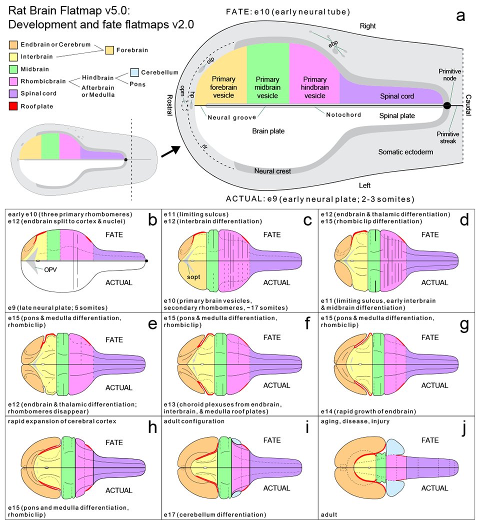
Bilateral flatmaps representing several stages of embryonic development of the rat nervous system, and the adult structure, beginning with the neural plate (a) (truncated caudally for the illustration as indicated by the inset), and progressing through eight representative embryonic stages (b-i) to adult (j). The lower half of each flatmap (left side, as shown) represents the actual embryonic (e) stage (or the adult); whereas the upper half (right side, as shown) represents the developmental fate of structures at a later stage. Major structures are color-coded as indicated by the color-key (top left) that also shows the relationships of the represented gray matter subdivisions. The area of the major subdivisions is proportional to the embryonic volume of corresponding gray matter (see Fig. 14 in Alvarez-Bolado & Swanson, 1996). The figure is based on a previous version (see Supporting Information 5 in Swanson, 2018) of an earlier original (see Figure 17 in Alvarez-Bolado & Swanson, 1996). For the purposes of illustration, structure labeling in b-j is simplified (for other labels see RtDevBF2 in Ai file Supporting Information 1, or the PDF file for RtDevBF2 in Supporting Information 2). Abbreviations: ebp, epibranchial placodes; hp, hypophysial placode; olp, olfactory placode; opm, oropharyngeal membrane; OPV, optic vesicle; rlr, rostrolateral ridge; sopt, optic sulcus.

As in BM4, each flatmap of brain development in RtDevBF2 is spatially registered to enable direct comparison of different developmental stages (they are also in register with RtBF5). The color-coding of major divisions is updated to conform with an updated scheme used here for RtBF5 (Figure 1), and the graphics are revised systematically for precise representation and alignment of tiles and lines representing each division and structure. Graphics and text properties are also refined to be consistent with those used here for RtBF5, and additional labeling is applied to fatemap structures to improve ease of identification. Layer arrangement of each developmental stage in the Ai file (Supporting Information 1) is refined systematically (Supporting Information 4). Additionally, as introduced for RtBF5, an optional light- or dark viewing mode is enabled by the inclusion of a dark and light background tile. A minor correction to version 1.0 in BM4 that is applied to the current version is depiction of the optic sulcus (sopt) on two fatemaps (actual stages e11 and e13) where it is present bilaterally but in BM4 was inadvertently hidden beneath graphical tiles on the lower half.

3.3. Mouse brain flatmap version 1.0 (MsBF1)

3.3.1. Mouse brain flatmap scaling

To facilitate direct comparison of mouse and rat brain data, flatmap backwards-compatibility, and future panmammalian comparative analyses, the MsBF1 template is scaled to match that used here for RtBF5 (and the previous version in BM4), and the hierarchy of gray matter divisions is organized according to the topographic arrangement used in BM4 (see Table C in Supporting Information 8 in Swanson, 2018). An additional rationale for equivalent scaling of the mouse and rat brain flatmaps is provided in a recent comparative analysis of the mouse and rat hippocampal formation to produce hippocampal cortex flatmaps (Swanson & Hahn, 2020). Using physical measurements of distances relative to bregma obtained from the BM4 and ARAv1 reference atlases, it was demonstrated that the relative spatial proportions of the mouse and rat hippocampal formation, and its major constituent subdivisions, is very similar (see Figure S1 in Swanson & Hahn, 2020), suggesting that a similar proportionality may apply to the mouse and rat brain in general.

3.3.2. Compatibility of mouse (ARAv1) and rat (BM4) brain reference atlas parcellation and nomenclature

A web-based version of the printed book version of ARAv1 (Dong, 2007) was made available in 2008 by the Allen Institute for Brain Science (http://mouse.brain-map.org/static/atlas). Design and construction of ARAv1 is described in the book (Dong, 2007) and also in a technical white paper for the web-based version that was published subsequently by the Allen Institute (Allen Institute for Brain Science, 2011), and is available on their website (http://help.brain-map.org/displav/mousebrain/Documentation). As noted in the introduction, although the listed hierarchical arrangement of brain divisions in ARAv1 differs from BM4, the nomenclatures are very similar because ARAv1 nomenclature followed predominantly BM3 nomenclature, that is largely consistent with BM4 nomenclature (Swanson, 2004; Swanson, 2018). A previous mouse brain atlas is cited as secondary nomenclature reference source for ARAv1 (Hof et al., 2000) (see text and appendix 3 in the documentation for the online version of ARAv1).

A concise list of nomenclature and parcellation differences between ARAv1 and BM4 is provided in Supporting Information 3. Excepting the retina and spinal cord (neither brain part was included in ARAv1), most of the differences are the result of a more coarse-grained parcellation in ARAv1 (resulting in fewer ARAv1 divisions overall, Figure 6) or to ARAv1 following a nomenclature and/or parcellation in BM3 that was revised in BM4. For instances where ARAv1 follows BM3 but differs from BM4, correspondence can be determined with reference to BM4 that includes detailed descriptions of revisions from the previous version. In addition, differences between ARAv1 and BM3 and/or BM4 are represented graphically on MsBFv1, including a layer that specifically represents differences between ARAv1 and BM4 (discussed in the subsequent section). An additional aid to determining gray matter region correspondence between ARAv1 and BM4 is a column of ordinal numbers included in Supporting Information 3 that are applied to the ARAv1 gray matter regions and correspond to numbers assigned to each gray matter region in BM4, indicating correspondence (where applicable).

Figure 6.

Comparison of the number of gray matter divisions for each depth of division of the central nervous system (CNS) according to its structural divisional hierarchy arranged topographically in Rat Brain Maps 4.0 (BM4) (Swanson, 2018), compared for the rat (based on BM4), and the mouse (based on the Allen Reference Atlas, ARAv1) (Dong, 2007). The upper chart (a) compares 9 depths of CNS divisions above the level of gray matter region (parent divisions) beginning with CNS at depth 1. The lower chart (b) shows the total numbers for all gray matter divisions (All divisions), and for the gray matter division categories of parent division (Parent), gray matter region (Region), and gray matter subregion (Subregion; including sub-subregion divisions, but excepting divisions that layers of cerebral and cerebellar cortical regions that apply similarly to rat and mouse). In general, ARAv1 has fewer gray matter divisions in each category (b) and at each depth of CNS division (a) compared to BM4, primarily due to a more coarse-grained parcellation. The retina (1 gray matter region) and spinal cord (22 gray matter regions) were not included in ARAv1 but were included in BM4; however, BM4 numbers for these divisions are included with the ARAv1 numbers here (and on MsBFv1 where they are present) to avoid exaggerating differences that were not due to these omissions. Conversely, to avoid understating differences, subregions that are laminar divisions of gray matter regions in the cerebral cortex and elsewhere (and present in both rat and mouse), are not included. Despite fewer ARAv1 gray matter divisions compared to BM4, the overall distribution is quite similar, reflecting a high-level of similarity in the underlying parcellation as represented in the reference atlases (see Supporting Information 3, and text for details).

All told, only six (out of 359, excepting the retina and spinal cord) gray matter regions in ARAv1 do not have a direct correspondence with gray matter divisions represented in BM3 or BM4, and four of these are described in the mouse brain atlas of Hof and colleagues (Hof et al., 2000) that, along with BM3 (Swanson, 2004), is cited in ARAv1 as one of two primary references. The four regions are the dorsal peduncular area (DP, mentioned in BM3, but not represented on the atlas maps); basolateral amygdalar nucleus ventral part (BLAv); subgeniculate nucleus (subG), and intermediate reticular nucleus (IRN). In rats, the DP was described previously as a subdivision of the infralimbic area (ILA) (Krettek & Price, 1977). Accordingly, here the DP is classified per BM4 nomenclature as a division of the cingulate region that includes the ILA (Swanson, 2018). Similarly, in mice, the BLAv and subG are both considered cytoarchitectural differentiations of another region: BLAv as a ventral differentiation of the BLA, and subG as a ventral differentiation of the lateral geniculate nucleus (Dong, 2007; Hof et al., 2000). Accordingly, following BM4 nomenclature, the BLAv is classified here as a division of the basolateral amygdalar nucleus, and the subG as a division of the ventral part of thalamus (Swanson, 2018). Lastly, the IRN is considered an intermediate differentiation of the parvicellular- and gigantocellular reticular nuclei (Dong, 2007; Hof et al., 2000) and is therefore classified as a division of the medulla (Swanson, 2018).

The two remaining ARAv1 gray matter regions without direct correspondence to BM3 or BM4 divisions, are the subparafascicular area (SPA) in the thalamus, and the hypothalamic paraventricular nucleus medial magnocellular part (PVHmm). The PVHmm was identified as a distinct gray matter region in mice in a focused study of the mouse PVH (Biag et al., 2012), but the SPA is defined less clearly. In ARAv1, the SPA is grouped with thalamic regions that in BM4 are classified as divisions of the ventral thalamic nuclei (gray matter parent division). However, as delineated in ARAv1, the SPA has partial spatial correspondence (overlap) with central medial- and intermediodorsal thalamic nuclei in BM4. A more recent example of SPA identification in mice also lacks clear definition of it (Hoerder-Suabedissen et al., 2018), and previously in rats a region referred to as the SPA was identified as a poorly defined division that contains part of the subparafascicular nucleus, but its relation to the latter is unclear (Faull & Mehler, 1985; Wang et al., 2006).

In addition to the six ARAv1 gray matter regions described above that differ from BM4 in terms of their parcellation and nomenclature, the coarser parcellation applied to some divisions in ARAv1 compared to BM4 includes ten regions described in BM3 (with direct correspondence to BM4) that were omitted from ARAv1, inadvertently or because of difficulty in identifying them during construction of ARAv1. These regions are identified in Supporting Information 3 and included for viewing in MsBF1 in a layer that shows BM4 comparative parcellation. Four of the 10 regions are described in BM3 and the mouse brain atlas of Hof and colleagues, per BM4 nomenclature they are (alphabetically): dorsal terminal nucleus of accessory optic tract (DT), medial accessory oculomotor nucleus (MAN), paratrigeminal nucleus (PAT), rostrolateral visual area (VISr1). The remaining 6 of 10 regions described in BM3, but not in the mouse brain atlas, are: interstitial nucleus of auditory nerve (IAN), interstitial nucleus of vestibular nerve (INV), medial terminal nucleus of accessory optic tract (MT), parabrachial nucleus lateral division extreme part (PBlex), parabrachial nucleus lateral division internal part (PBli), superior salivatory nucleus (SSN). Identification of these differences, and the others described in this section, between ARAv1 and BM4 serves to clarify compatibility between these two reference atlases and provides information that may be useful for future possible revisions.

3.3.3. Flatmap representation of correspondences and differences between MsBF1 and RtBF5

As described in the earlier results section for RtBF5, the general design and format of MsBF1 is the same as RtBF5. For details of the general design and format refer to the earlier section, and for an annotated list of the Ai file layers for MsBF1 see Supporting Information 4. Several design features implemented for MsBF1 enable identification of correspondences and differences between MsBF1 and RtBF5 (and therefore between ARAv1 and BM4). These include a comparative parcellation layer in MsBF1 that represents differences between ARAv1 and BM4. When visible, the comparative layer highlights (with magenta lines and fills, and gray text) gray matter regions and subregions represented in BM4 that differ in their parcellation from ARAv1. For gray matter regions that were omitted from ARAv1 but are likely present (see preceding section), this layer can be used to represent them selectively on MsBF1.

For ease of locating gray matter divisions (subregions, regions, and parent divisions) on MsBF1, the tiles (filled shapes) representing them are named by their abbreviation and listed alphabetically (as in RtBF5), see Supporting Information 3. Additionally, to help identify nomenclature differences, where parcellation between ARAv1 and BM4 is equivalent, but there is a difference in name only, the BM4 abbreviation is appended in parenthesis following the ARAv1 abbreviation. For example, the gray matter region named globus pallidus internal segment (GPi) in ARAv1, is named medial globus pallidus (GPm) in BM4, but the regions are otherwise considered equivalent. Accordingly, the listed entry for the tile representing GPi on MsBF1 is named “GPi (GPm in BM4)”. Differences in hierarchical assignment are indicated similarly. For example, in BM4 the lateral septal nucleus rostral part (LSr) is a parent division, but in ARAv1 the LSr is not subdivided and is therefore represented on MsBF1 as a gray matter region. Accordingly, the entry for the tile representing LSr on MsBF1 is named “LSr (parent in BM4)”. Similar parenthesized information is also appended to other entries to facilitate comparison between BM4 and ARAv1 when using MsBF1.

Additional graphical design features applied to MsBF1 are used to identify correspondences and differences between ARAv1 and BM4 and/or BM3. In a similar manner to information in parenthesis being appended to the name of each division tile to indicate a difference in division name but correspondence in parcellation, so too on the flatmap ARAv1 abbreviations to which this applies are shown in parenthesis (GPi, for example, as noted above). To identify parcellation differences at the level of gray matter regions and subregions a different approach is used involving differences in tile color. The default tile color is yellow, and all yellow tiles on MsBF1 indicate an equivalent parcellation between ARAv1 and BM4 (although in some instances, explained below, the shape of corresponding tiles differs). Gray tiles indicate ARAv1 and BM3 parcellation equivalence, but a difference from BM4 (for example parcellation of the anterior olfactory nucleus, AON). Magenta tiles indicate a difference in parcellation between ARAv1 and both BM3 and BM4, primarily due to coarser granularity. For example the LSr, as noted above, and all gray matter regions of the spinal cord because the spinal cord was not included in ARAv1.

For instances where the shape of a tile differs between MsBF1 and RtBF5, but not the underlying atlas parcellation, the difference is represented in the BM4 comparative parcellation layer only. Examples include tiles for regions of the cerebral cortex that differ in shape between MsBF1 and RtBF5 because of different representation of atlas level contours for BM4 and ARAv1, with which they are aligned. Lastly, cyan tiles indicate a parcellation that is ARAv1-specific (it has no comparable counterpart in either BM3 or BM4) (see the preceding section). The combination of different tile coloring, information appended to individual layer names, and comparative BM4 parcellation, provide visual aids to help identify correspondences and differences between MsBF1 and RtBF5. These design feature implemented for MsBF1 are also supported by tables that provide additional information (Supporting Information 3).

3.3.4. Flatmap adaptability for novel parcellations derived from experimental data

Brain flatmaps, in addition to providing diagrammatic representation of brain architecture for comparative analysis in general, can also be used to represent the results of experiments. Using the present brain flatmaps, data can be mapped to the original parcellation schema corresponding to the underlying brain reference atlases, or if data suggest an alternate parcellation schema then it can be delineated with reference to the original parcellation. To illustrate this using MsBF1, we provide two examples of experiment-based parcellation schemas. The first example is a refined caudoputamen (CP) parcellation based on network analysis of mouse cerebral cortex to CP connection data derived from anterograde pathway-tracing experiments (Hintiryan et al., 2016). Subnetworks were identified in the CP by a combination of community detection network analysis applied to the incidence matrix of cerebral cortex to CP connection data, and centrality analysis applied to CP axonal labeling, using a square grid-based CP reference at a spatial resolution of 22.5 μm². Three levels of the CP along its longitudinal axis were analyzed: rostral, intermediate, and caudal. Network analysis applied to data for each level identified a total of 11 second-level subdivisions, termed communities, and 25 third-level subdivisions, termed domains (Figure 7a).

Figure 7.

Flatmap adaptability to novel parcellation schemas based on experimental data. Two examples, using MsBF1, illustrate how the present brain flatmaps can be adapted to represent novel parcellations. The first example (a) represents a refined parcellation for the caudoputamen (CP) based on network analysis of axonal connections from the cerebral cortex to the CP (Hintiryan et al., 2016). The second example (b) represents a refined parcellation for hippocampal regions based on a combination of gene-expression and network analysis (Bienkowski et al., 2018). The hippocampal divisions were mapped to the parcellation represented on MsBF1, and also with respect to atlas level contours for the cerebral cortex corresponding to ARAv1 (shown in purple on the right side of (b), that also shows the retrohippocampal region that is the other major division of the hippocampal formation). The insets at lower left show the general location of the regions shown in (a) and (b). The table at lower right shows the divisional hierarchy underlying each novel parcellation schema, and ARAv1 atlas levels for the hippocampal divisions. See text for additional information. Abbreviations shown in red text in (b) (upper right side) are defined in Supporting Information 3. Abbreviations for (a) and upper part of table: cd, central dorsal; cvl, central ventrolateral; cvm, central ventromedial; d, dorsal; dl, dorsolateral; dm, dorsomedial; ext, extreme; i, intermediate; im, intermedial; imd, intermedial dorsal (applies to CPi.dl.imd); imd, intermediate dorsal (applies to CPr.imd); imv, intermedial ventral (applies to CPi.vl.imv); imv, Intermediate ventral (applies to CPr.imv); l, lateral; ls, lateral strip; r, rostral; v, ventral; vm, ventromedial; vt, ventral tip. Abbreviations for (b) and lower part of table: CA1-3, Ammon’s horn (cornu Ammonis in Latin) Field 1, 2, or 3; CAldc, CA1 dorsal, caudal part; CAldr, CA1 dorsal, rostral part; CAlvv, CA1 ventral tip; CA3dd, CA3 rostral-dorsal tip; CA3vv, CA3 ventral tip; dc, dorsal caudal; dd, dorsal tip; DG, dentate gyrus; ic, intermediate caudal; id, intermediate dorsal; pod, dorsal polymorph layer; pov, ventral polymorph layer; ProSUB, prosubiculum; SUB, subiculum; SUBdd, dorsal subiculum, dorsal part (tip); SUBdv, dorsal subiculum, ventral part (tip); SUBvv, ventral subiculum, ventral part (tip).

The second example of a novel flatmap parcellation for MsBF1 is based on the results of pathway-tracing experiments of hippocampal regions, delineated by differential gene-expression, and subsequently by network analysis applied to pathway-tracing data for intrahippocampal connections (Bienkowski et al., 2018). Network analysis of the adjacency matrix formed by intrahippocampal connection data across a range of network resolutions (variation of network resolution parameter gamma), revealed prominent consensus clusters at three of them, suggesting a 3-tier hierarchy of nested subdivisions. Figure 7b shows the lowest level subdivisions mapped to MsBF1 hippocampal regions, and to corresponding cerebral cortex atlas levels contours based on ARAv1. For three atlas levels (80-82) the contours are adjusted slightly to conform with a previous correction to an ARAv1 error whereby the ventral subiculum’s rostral tip is indicated correctly on atlas level 79, and caudally on atlas levels 83-91, but was omitted from the intervening atlas levels (Swanson & Hahn, 2020) (in Supporting Information 1 the corresponding contour line segments are colored red).

Each of these two examples illustrate how MsBF1 can be adapted to represent alternative parcellation schemas— the same basic strategy could be applied also to the other brain flatmaps presented here. For reference, the two novel parcellation schemas are included in the MsBF1 Ai file (Supporting Information 1) as separate layers, with nested sublayers arranged according to the identified subdivisions (Supporting Information 4). As illustrated in Figure 4, for the cortical layer markers included with RtBF5, once a parcellation is instantiated on the flatmap it can be recolored to represent quantitative and/or qualitative differences in data, providing utility and flexibility for future comparative analyses.

3.4. Human brain flatmap version 3.0. (HuBF3)

The graphical design and format of HuBF3 in general follows MsBF1, RtBF5, and RtDevBF2. Upgrades applied to those flatmaps that also apply to HuBF3 include streamlined graphics and text, improved point-alignment of graphical elements (lines and tiles), and other visual enhancements including an optional dark background for optimal viewing. Updates to the second version of the human brain flatmap (included in BM4) that are applied to HuBF3, include: 1) clarification of parcellation of regions of the hippocampal formation and basolateral amygdalar complex (following BM4 parcellation and nomenclature for the rat); 2) revised delineation of the tenia tecta, anterior olfactory area, and indusium griseum rostrally (where it is adjacent to the tenia tecta) to conform with similar revisions to delineation of these regions for RtBF5; 3) clearer differentiation of the cortical subplate; 4) representation of the retina. In addition to these updates, graphical presentation of HuBF3 is enhanced with additional coloration of major brain parts that are similarly represented for the other brain flatmap categories presented here (Figure 8).

Figure 8.

A flatmap representation of the adult human brain (a) showing on the upper half (right side of brain) Brodmann’s areal parcellation and associated numbering schema for divisions of the cerebral cortex, and on the lower half (left side of brain) primary sulci. The nested cortical subplate is outlined in green on the upper half. Also represented are major structural divisions of the brain, represented differently on either side for the purposes of illustration; their structural hierarchical relationships are indicated by a color-coded tree. Additional divisional parcellation is represented by the inset (b) for the basolateral amygdalar complex (BLX), and for selected divisions of the hippocampal formation. The present version of the human brain map (version 3) is based on an earlier (second) version (Swanson, 2018). See text for additional information. Abbreviations for (a): 6b, isocortical layer 6b; AOA, anterior olfactory area; CA, Ammon’s horn (cornu Ammonis in Latin); CBN, cerebellar nuclei; CLA, claustrum; COX, cortical amygdalar complex; DG, dentate gyrus; EP, endopiriform nucleus; IG, indusium griseum; INS, insular region; MB, midbrain; OB, olfactory bulb; PAL, pallidum; SBC, subicular complex; STR, striatum; TG, tegmentum; TT, tenia tecta. Abbreviations for (b): BLA, basolateral amygdala nucleus; BMA, basomedial amygdala nucleus; CA1-3, CA fields 1-3; d, dorsal; LA, lateral amygdala nucleus; m, medial; PARA, parasubiculum; POST, postsubiculum; PRE, presubiculum; SUB, subiculum; v, ventral.

Terminology for HuBF3 follows the terminology used in BM4 for the second version that was updated to conform with a current lexicon of human neuroanatomical terminology (Swanson, 2015a). Additionally, clarification of hippocampal formation parcellation for HuBF3 includes additional identification and labeling of numbered Brodmann areas to conform with an updated view of Brodmann areas (see Supporting Information Table S1 in Swanson & Hof, 2019) based on correspondences drawn between rat and human (see Supplementary Information Figure S2 in Bota et al., 2015). Accordingly, and as noted (but not labeled on the human brain flatmap) in BM4, the following numbered Brodmann areas are identified and labeled on HuBF3: Brodmann area 34 (included with area 28 in the entorhinal area), area 27 (presubiculum), and area 48 (postsubiculum). Also labeled is Brodmann area 49 that was identified by Brodmann in non-human animals as the parasubicular area (Swanson, 2015a), corresponding in rat to the parasubiculum (Bota et al., 2015; Swanson, 2018; Swanson & Hof, 2019), and so indicated on HuBF3 as a division of the subicular complex (together with Brodmann area 27 and 48) (Figure 8b). Area 50, identified and numbered by Brodmann in non-human animals, in rat corresponds to temporal associations areas, but Brodmann remained uncertain of its structural classification and drew no human correspondence—area 50 is the only one of the fifty-two Brodmann-numbered areas not represented on HuBF3 (Simic & Hof, 2015; Swanson, 2015a; Swanson, 2018; Swanson & Hof, 2019).

The graphical enhancements noted above that are applied to HuBF3 are also supported by enhanced layering in the Ai file (Supporting Information 1) that is described in Supporting Information 4 for 24 layers to a nested depth of 4 levels. Enhancements applied to the Ai file layering to facilitate use of HuBF3 are similar to those applied to the other flatmap categories presented here; they include naming of individual tiles representing each gray matter division by the abbreviation of the division name, and arrangement of tiles in alphabetical or numerical order (for example for tiles representing Brodmann-numbered areas of the cerebral cortex).

4. Discussion

Mice are currently the most used vertebrate animals in neuroscience research, yet for most of the 20^th century the same could be said of rats (Ellenbroek & Youn, 2016). While official (government) research use statistics are not provided in the United States for these animals, a 2016 United Kingdom government report on biomedical research for the years 2006-2015 (https://www.gov.uk/government/statistics/statistics-of-scientific-procedures-on-living-animals-great-britain-2015) found that mice accounted for 61% of animals used in experimental procedures, compared to 12% for rats (and 7% for birds, and less for other animals). Despite the current dominance of mice as research animals in neuroscience, and the nearly 3-decade availability of a brain flatmap for the rat based on a corresponding reference atlas (Brain Maps 1, BM1) (Swanson, 1992), a comparable mouse brain flatmap was not available previously. To address this, here we have provided version 1.0 of a flatmap for the mouse brain (MsBF1) based on a corresponding mouse brain reference atlas (ARAv1) (Dong, 2007).

Our principal reason for selecting ARAv1 as the basis for MsBF1 is (as considered earlier) a nearly complete direct correspondence in nomenclature and parcellation between ARAv1 and the fourth (current) version of a rat brain reference atlas (Brain Maps 4.0, BM4) (Swanson, 2018), as a result of the previous version (BM3) (Swanson, 2004) being used as the main reference model for ARAv1. Furthermore, matching MsBF1 to the present updated rat brain flatmap (RtBF5) with respect to flatmap scaling, and aligning both to BM4 with respect to the nomenclature and topographic arrangement of gray matter divisions used in BM4 (Supporting Information 3), following their previous application to the human nervous system (Swanson, 2015a), support the goal (expressed in BM4) of developing a “…panmammalian (and ultimately a panvertebrate) textual and spatial nomenclature for describing nervous system structural organization, while incorporating differentiations of the basic plan characteristic of each species.” (Swanson, 2018). The enhanced rat brain development flatmaps (RtDevBF2) and human brain flatmap (HuBF5) presented here, that also align with BM4, and are presented together with MsBF1 and RtBF5 (Supporting Information 1), add further support to this goal.

The utility of 3-D reconstruction of brain-mapped data was recognized in BM1 that included 73 spatially aligned digital atlas level maps created in Adobe Illustrator (Swanson, 1992), as a step toward the future goal of a fully realized 3D brain atlas. Currently, efforts continue toward the challenging dual-goals of constructing 3-D brain reference atlases and creating the tools and techniques to map brain data to them efficiently and with high fidelity. Notable recent efforts include those by the Allen Institute, for human (Ding et al., 2016; Hawrylycz et al., 2012; Shen et al., 2012; Zeng et al., 2012) and mouse (Oh et al., 2014; Allen Mouse Common Coordinate Framework version 3, 2017, described in a technical white paper: http://help.brain-map.org/download/attachments/2818169/MouseCCF.pdf), and efforts by other groups (for example Goubran et al., 2019; Ni et al., 2020; Niedworok et al., 2016) (see also an online compendium resource published by the International Neuroinformatics Coordinating Facility (INCF): https://scalablebrainatlas.incf.org/index.php). However, even as these efforts bring us closer to achieving desired 3-D brain mapping goals, the utility of 2-D brain flatmaps as a comparative tool may well increase rather than diminish, because they provide a relatively straightforward way to summarize brain data in a form that is readily grasped, and in a format that is easily distributed.

Given the utility of brain flatmaps for summarizing and comparing brain data, in the remaining part of the discussion we consider how they may be used as a foundation for a web-based brain flatmap viewer and comparative analysis platform that enables on-demand flatmap visualization of brain data—a goal envisioned previously (Brown & Swanson, 2015), and rudimentarily realized (Kim et al., 2017), that we are continuing to work toward. As proof-of-concept for our strategy to achieve this, we refer to our studies of mouse brain connectomics, collectively referred to as the mouse connectome project (MCP). The MCP currently encompasses multiple levels of granularity from individual neurons to regional brain circuits. To date, region-level granularity has received most attention (Bienkowski et al., 2019; Bienkowski et al., 2018; Hintiryan et al., 2016; Hintiryan et al., 2012; Zingg et al., 2018; Zingg et al., 2014), and is used here to instantiate the flatmap visualization workflow, using data from a recent study of claustrum connections (Zingg et al., 2018).

The typical starting point for analysis of brain circuits that are formed by axonal connections between gray matter regions is a pathway-tracing experiment. For the MCP, we have used several different anterograde and retrograde pathway-tracing methods, singly or in combination, to investigate brain circuit organization. The basic methodological sequence is as follows: 1) pathway-tracer injection(s) targeted to region(s) of interest, 2) brain tissue histological processing and serial sectioning, 3) digital imaging of brain sections, 4) warping and registration of digitally imaged sections to ARAv1 using a Nissl-stained reference series, 5) signal-to-noise optimization, 6) manual or automated grid-based analysis of the processed images to obtain a measure of signal (based fundamentally on pixel count) for each ARAv1-defined gray matter region and selected atlas levels. For regions of particular interest, subsequent analysis at finer levels of granularity (higher spatial resolution) may be performed by increasing the analysis grid resolution.

To generate a brain flatmap representation (here for MsBF1) of the experimental data at the level of gray matter regions, the next step is data aggregation across ARAv1 atlas levels for each gray matter region. With that accomplished, the data can then be visualized on MsBF1 (for example as a heatmap). Following data collection and preparation (steps 1-6 in the methodological sequence described above), the flatmap visualization process has three basic steps (Figure 9). To automate the visualization step, MsBF1 could be implemented as a scalable vector graphics (SVG) object with a tagged coordinate system used to enable matching of the region-aggregated input data to corresponding SVG coordinates representing each gray matter region (or other user-defined parcellation represented in relation to the reference atlas parcellation). Approaches similar to this, using SVG and a variety of other software-based approaches, are well established for geographic cartography (Lienert et al., 2012).

Figure 9.

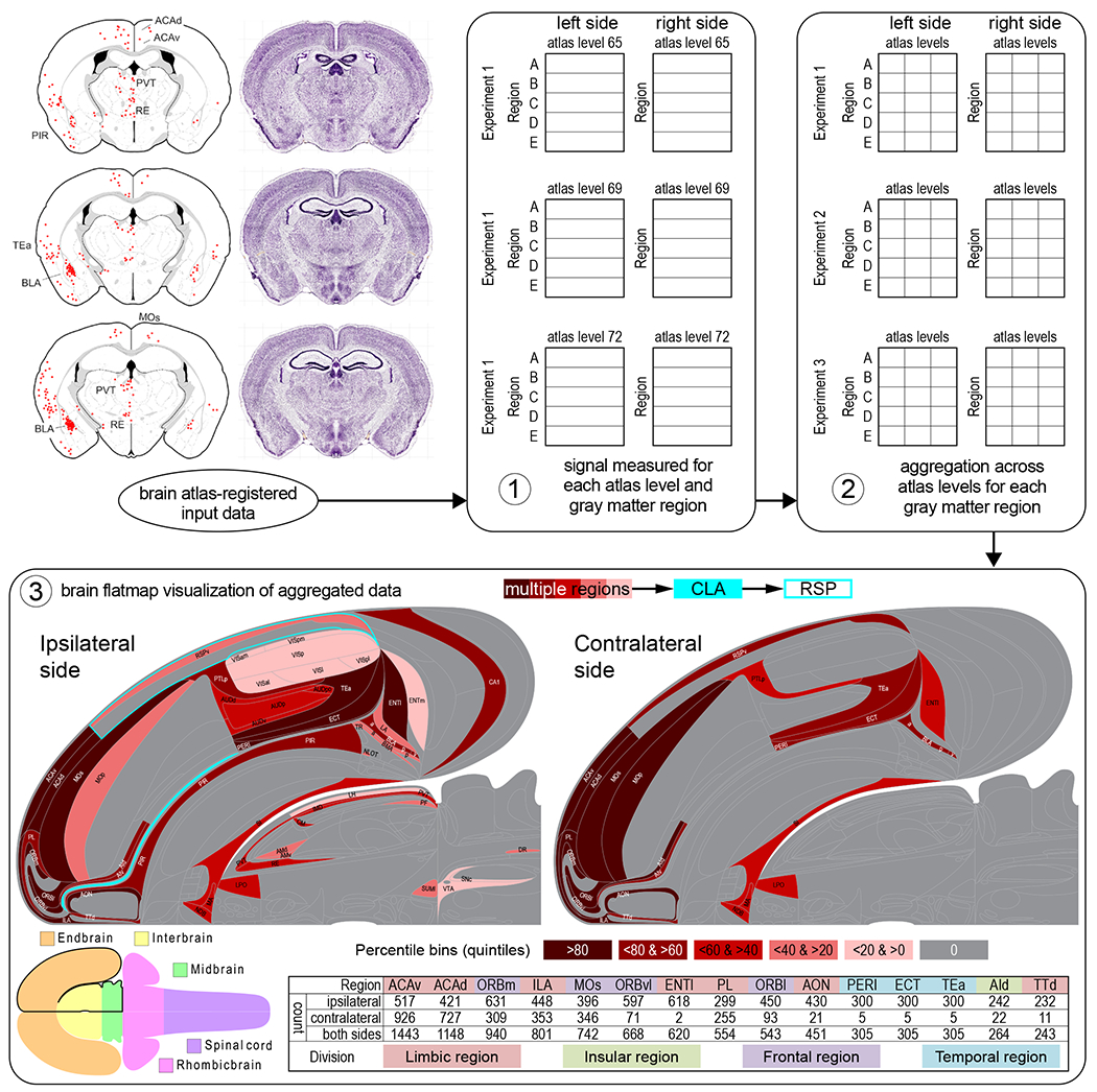
A conceptual brain flatmap visualization workflow. Initial input to the brain flatmap visualization workflow is tabulated experimental data representing measured values (automated pixel count, or cell count that is either manual or based on a thresholding algorithm applied to pixel count) corresponding to signal (for example a fluorescent reporter molecule) detected in brain tissue sections after histological processing, digital imaging, registration to a brain reference atlas (in this example a computer graphics version of the Allen Reference Atlas version 1 (ARAv1), Dong, 2007), and image processing to achieve optimal signal-noise ratio. Following data input, step 1 of the workflow analysis generates an annotated output recording data location by ARAv1 atlas level and by gray matter region (according to boundaries representing ARAv1 parcellation). In step 2, the data are aggregated across atlas levels for each gray matter region, to give an average value for each region; aggregation may also be performed across experiments (as indicated). In step 3, the aggregated region-specific data are visualized (for example as a heatmap as shown) on a scalable vector graphic implementation of the brain flatmap using a back-end coordinate system with tags applied to each coordinate-defined area to enable matching to gray matter regions. The example data shown here were reported previously (Zingg et al., 2018—Atlas Level maps (top left) reproduced from Figure 5, and flatmap visualization based on data for Animal 1 in Table 3); they represent sites of input to claustrum neurons that send monosynaptic projections to the retrosplenial area, determined by a combinatorial and conditional virus-based pathway-tracing strategy (Zingg et al., 2018). A monochrome heatmap represents positive data in five percentile bins (quintiles) calculated separately for connections ipsilateral and contralateral to the side targeted. The brain schematic at lower left represents major divisions of the central nervous system (see also Figure 1). The table at lower right lists cell counts for regions in the top 25% for total cell count, arranged from high to low, and showing counts for the targeted side (ipsilateral), contralateral side, and both sides (total). Background colors applied to the region abbreviations correspond to the color-coded CNS divisions below the table. For abbreviations see Supporting Information 3.

The example we have given here shows brain flatmap visualization of neural connection data. However, the same basic strategy could be applied to represent other types of data, such as patterns of gene expression, neural activity, or sites associated with gain or loss of function; more complex combinatorial data representations are also possible. The demand for such an approach is evident from recent work that used version 3 of the rat brain flatmap in BM3 (Swanson, 2004) to display mouse brain data (Kim et al., 2017), and from ongoing mouse brain mapping efforts by the Allen Institute (Chon et al., 2019). Furthermore, while the example given here is rooted in structural differentiations that define gray matter regions, a coordinate-based approach could be developed. For MsBF1, a step in this direction is demonstrated in Figure 7b that shows data mapping to both gray matter region and to ARAv1 atlas levels for the cerebral cortex. To enable coordinate mapping of 3-D space (brain) to 2-D space (brain flatmap), one possible approach combines a coordinate system for two dimensions (medial-lateral and dorsal-ventral axes) with mapping to each atlas level representing the third dimension (rostral-caudal axis) (see Fig. 12 and discussion in Swanson & Hahn, 2020). Such approaches are likely to have increasing relevance in basic research as coordinate-based approaches to mapping brain data continue to gain ground (Khan, 2013; Khan et al., 2018).

Brain mapping resources provided open access, and the goal of a pan-mammalian nomenclature for the nervous system, are both recognized for their potential value to neuroscience research (Swanson, 2015b; Swanson, 2018). The brain flatmaps presented here support this ethos, and they also support the acquisition and dissemination of neuroscientific knowledge about the structure and function of the brain and nervous system.

References

- Alvarez-Bolado G, & Swanson LW (1996). Developmental brain maps: structure of the embryonic rat brain. Elsevier: Publisher description; http://www.loc.gov/catdir/enhancements/fy0601/96015900-d.html [Google Scholar]
- Biag J, Huang Y, Gou L, Hintiryan H, Askarinam A, Hahn JD, Toga AW, & Dong HW (2012). Cyto- and chemoarchitecture of the hypothalamic paraventricular nucleus in the C57BL/6J male mouse: a study of immunostaining and multiple fluorescent tract tracing. J Comp Neurol, 520(1), 6–33. 10.1002/cne.22698 [DOI] [PMC free article] [PubMed] [Google Scholar]
- Bienkowski MS, Benavidez NL, Wu K, Gou L, Becerra M, & Dong HW (2019). Extrastriate connectivity of the mouse dorsal lateral geniculate thalamic nucleus. J Comp Neurol, 527(9), 1419–1442. 10.1002/cne.24627 [DOI] [PMC free article] [PubMed] [Google Scholar]
- Bienkowski MS, Bowman I, Song MY, Gou L, Ard T, Cotter K, Zhu M, Benavidez NL, Yamashita S, Abu-Jaber J, Azam S, Lo D, Foster NN, Hintiryan H, & Dong HW (2018). Integration of gene expression and brain-wide connectivity reveals the multiscale organization of mouse hippocampal networks. Nat Neurosci, 21(11), 1628–1643. 10.1038/s41593-018-0241-y [DOI] [PMC free article] [PubMed] [Google Scholar]
- Bota M, Sporns O, & Swanson LW (2015). Architecture of the cerebral cortical association connectome underlying cognition. Proc Natl Acad Sci U S A, 112(16), E2093–2101. 10.1073/pnas.1504394112 [DOI] [PMC free article] [PubMed] [Google Scholar]
- Brown RA, & Swanson LW (2015). Golgi: interactive online brain mapping. Front Neuroinform, 9, 26 10.3389/fninf.2015.00026 [DOI] [PMC free article] [PubMed] [Google Scholar]
- Chon U, Vanselow DJ, Cheng KC, & Kim Y (2019). Enhanced and unified anatomical labeling for a common mouse brain atlas. Nat Commun, 10(1), 5067 10.1038/s41467-019-13057-w [DOI] [PMC free article] [PubMed] [Google Scholar]
- Ding SL, Royall JJ, Sunkin SM, Ng L, Facer BA, Lesnar P, Guillozet-Bongaarts A, McMurray B, Szafer A, Dolbeare TA, Stevens A, Tirrell L, Benner T, Caldejon S, Dalley RA, Dee N, Lau C, Nyhus J, Reding M, Riley ZL, Sandman D, Shen E, van der Kouwe A, Varjabedian A, Wright M, Zollei L, Dang C, Knowles JA, Koch C, Phillips JW, Sestan N, Wohnoutka P, Zielke HR, Hohmann JG, Jones AR, Bernard A, Hawrylycz MJ, Hof PR, Fischl B, & Lein ES (2016). Comprehensive cellular-resolution atlas of the adult human brain. J Comp Neurol, 524(16), 3127–3481. 10.1002/cne.24080 [DOI] [PMC free article] [PubMed] [Google Scholar]
- Dong HW (2007). The Allen Reference Atlas, (Book + CD-ROM): a digital color brain atlas of the C57BL/6J male mouse. Wiley. [Google Scholar]
- Ellenbroek B, & Youn J (2016). Rodent models in neuroscience research: is it a rat race? Dis Model Mech, 9(10), 1079–1087. 10.1242/dmm.026120 [DOI] [PMC free article] [PubMed] [Google Scholar]
- Faull RLM, & Mehler WR (1985). Thalamus In: The rat nervous system (Vol. 1). Academic Press. [Google Scholar]
- Goubran M, Leuze C, Hsueh B, Aswendt M, Ye L, Tian Q, Cheng MY, Crow A, Steinberg GK, McNab JA, Deisseroth K, & Zeineh M (2019). Multimodal image registration and connectivity analysis for integration of connectomic data from microscopy to MRI. Nat Commun, 10(1), 5504 10.1038/s41467-019-13374-0 [DOI] [PMC free article] [PubMed] [Google Scholar]
- Hahn JD, Sporns O, Watts AG, & Swanson LW (2019). Macroscale intrinsic network architecture of the hypothalamus. Proc Natl Acad Sci U S A, 116(16), 8018–8027. 10.1073/pnas.1819448116 [DOI] [PMC free article] [PubMed] [Google Scholar]
- Hahn JD, & Swanson LW (2015). Connections of the juxtaventromedial region of the lateral hypothalamic area in the male rat. Front Syst Neurosci, 9(66), 66 10.3389/fnsys.2015.00066 [DOI] [PMC free article] [PubMed] [Google Scholar]
- Hawrylycz MJ, Lein ES, Guillozet-Bongaarts AL, Shen EH, Ng L, Miller JA, van de Lagemaat LN, Smith KA, Ebbert A, Riley ZL, Abajian C, Beckmann CF, Bernard A, Bertagnolli D, Boe AF, Cartagena PM, Chakravarty MM, Chapin M, Chong J, Dalley RA, David Daly B, Dang C, Datta S, Dee N, Dolbeare TA, Faber V, Feng D, Fowler DR, Goldy J, Gregor BW, Haradon Z, Haynor DR, Hohmann JG, Horvath S, Howard RE, Jeromin A, Jochim JM, Kinnunen M, Lau C, Lazarz ET, Lee C, Lemon TA, Li L, Li Y, Morris JA, Overly CC, Parker PD, Parry SE, Reding M, Royall JJ, Schulkin J, Sequeira PA, Slaughterbeck CR, Smith SC, Sodt AJ, Sunkin SM, Swanson BE, Vawter MP, Williams D, Wohnoutka P, Zielke HR, Geschwind DH, Hof PR, Smith SM, Koch C, Grant SGN, & Jones AR (2012). An anatomically comprehensive atlas of the adult human brain transcriptome. Nature, 489(7416), 391–399. 10.1038/nature11405 [DOI] [PMC free article] [PubMed] [Google Scholar]
- Hintiryan H, Foster NN, Bowman I, Bay M, Song MY, Gou L, Yamashita S, Bienkowski MS, Zingg B, Zhu M, Yang XW, Shih JC, Toga AW, & Dong HW (2016). The mouse cortico-striatal projectome. Nat Neurosci, 19(8), 1100–1114. 10.1038/nn.4332 [DOI] [PMC free article] [PubMed] [Google Scholar]
- Hintiryan H, Gou L, Zingg B, Yamashita S, Lyden HM, Song MY, Grewal AK, Zhang X, Toga AW, & Dong HW (2012). Comprehensive connectivity of the mouse main olfactory bulb: analysis and online digital atlas. Front Neuroanat, 6, 30 10.3389/fnana.2012.00030 [DOI] [PMC free article] [PubMed] [Google Scholar]
- Hoerder-Suabedissen A, Hayashi S, Upton L, Nolan Z, Casas-Torremocha D, Grant E, Viswanathan S, Kanold PO, Clasca F, Kim Y, & Molnar Z (2018). Subset of cortical layer 6b neurons selectively innervates higher order thalamic nuclei in mice. Cereb Cortex, 28(5), 1882–1897. 10.1093/cercor/bhy036 [DOI] [PMC free article] [PubMed] [Google Scholar]
- Hof PR, Young WG, Bloom FE, Belichenko PV, & Celio MR (2000). Comparative cytoarchitectonic atlas of the C57BL/6 and 129/Sv mouse brains. Elsevier. [Google Scholar]
- Josephson S (2008). Keeping your readers’ eyes on the screen: an eye-tracking study comparing sans serif and serif typefaces. Visual Communication Quarterly, 15(1-2), 67–79. 10.1080/15551390801914595 [DOI] [Google Scholar]
- Khan AM (2013). Controlling feeding behavior by chemical or gene-directed targeting in the brain: what’s so spatial about our methods? Front Neurosci, 7, 182 10.3389/fnins.2013.00182 [DOI] [PMC free article] [PubMed] [Google Scholar]
- Khan AM, Perez JG, Wells CE, & Fuentes O (2018). Computer vision evidence supporting craniometric alignment of rat brain atlases to streamline expert-guided, first-order migration of hypothalamic spatial datasets related to behavioral control. Front Syst Neurosci, 12, 7 10.3389/fnsys.2018.00007 [DOI] [PMC free article] [PubMed] [Google Scholar]
- Kim Y, Yang GR, Pradhan K, Venkataraju KU, Bota M, Garcia Del Molino LC, Fitzgerald G, Ram K, He M, Levine JM, Mitra P, Huang ZJ, Wang XJ, & Osten P (2017). Brain-wide maps reveal stereotyped cell-type-based cortical architecture and subcortical sexual dimorphism. Cell, 171(2), 456–469, e422 10.1016/j.cell.2017.09.020 [DOI] [PMC free article] [PubMed] [Google Scholar]
- Krettek JE, & Price JL (1977). The cortical projections of the mediodorsal nucleus and adjacent thalamic nuclei in the rat. J Comp Neurol, 171(2), 157–191. 10.1002/cne.901710204 [DOI] [PubMed] [Google Scholar]
- Lienert C, Jenny B, Schnabel O, & Hurni L (2012). Current trends in vector-based internet mapping: a technical review In Peterson MP (Ed.), Online Maps with APIs and Web Services (1st ed., pp. 23–26). Springer-Verlag. [Google Scholar]
- Ni H, Tan C, Feng Z, Chen S, Zhang Z, Li W, Guan Y, Gong H, Luo Q, & Li A (2020). A robust image registration interface for large volume brain atlas. Sci Rep, 10(1), 2139 10.1038/s41598-020-59042-y [DOI] [PMC free article] [PubMed] [Google Scholar]
- Niedworok CJ, Brown AP, Jorge Cardoso M, Osten P, Ourselin S, Modat M, & Margrie TW (2016). aMAP is a validated pipeline for registration and segmentation of high-resolution mouse brain data. Nat Commun, 7, 11879 10.1038/ncomms11879 [DOI] [PMC free article] [PubMed] [Google Scholar]
- Oh SW, Harris JA, Ng L, Winslow B, Cain N, Mihalas S, Wang Q, Lau C, Kuan L, Henry AM, Mortrud MT, Ouellette B, Nguyen TN, Sorensen SA, Slaughterbeck CR, Wakeman W, Li Y, Feng D, Ho A, Nicholas E, Hirokawa KE, Bohn P, Joines KM, Peng H, Hawrylycz MJ, Phillips JW, Hohmann JG, Wohnoutka P, Gerfen CR, Koch C, Bernard A, Dang C, Jones AR, & Zeng H (2014). A mesoscale connectome of the mouse brain. Nature, 508(7495), 207–214. 10.1038/nature13186 [DOI] [PMC free article] [PubMed] [Google Scholar]
- Shen EH, Overly CC, & Jones AR (2012). The Allen Human Brain Atlas: comprehensive gene expression mapping of the human brain. Trends Neurosci, 35(12), 711–714. 10.1016/j.tins.2012.09.005 [DOI] [PubMed] [Google Scholar]
- Simic G, & Hof PR (2015). In search of the definitive Brodmann’s map of cortical areas in human. J Comp Neurol, 523(1), 5–14. 10.1002/cne.23636 [DOI] [PubMed] [Google Scholar]
- Swanson LW (1992). Brain Maps: Structure of the Rat Brain. Elsevier. [Google Scholar]
- Swanson LW (1995). Mapping the human brain: past, present, and future. Trends Neurosci, 78(11), 471–474. [DOI] [PubMed] [Google Scholar]
- Swanson LW (1998). Brain maps: structure of the rat brain: a laboratory guide with printed and electronic templates for data, models, and schematics (2nd ed.). Elsevier. [Google Scholar]
- Swanson LW (2004). Brain maps: structure of the rat brain: a laboratory guide with printed and electronic templates for data, models, and schematics (3rd ed.). Elsevier. [Google Scholar]
- Swanson LW (2015a). Neuroanatomical terminology : a lexicon of classical origins and historical foundations. Oxford University Press. [Google Scholar]
- Swanson LW (2015b, Oct 15). Brain maps online: toward open access atlases and a pan-mammalian nomenclature. J Comp Neurol, 523(15), 2272–2276. 10.1002/cne.23788 [DOI] [PubMed] [Google Scholar]
- Swanson LW (2018). Brain maps 4.0-structure of the rat brain: an open access atlas with global nervous system nomenclature ontology and flatmaps. J Comp Neurol, 526(6), 935–943. 10.1002/cne.24381 [DOI] [PMC free article] [PubMed] [Google Scholar]
- Swanson LW, & Bota M (2010). Foundational model of structural connectivity in the nervous system with a schema for wiring diagrams, connectome, and basic plan architecture. Proc Natl Acad Sci U S A, 707(48), 20610–20617. [DOI] [PMC free article] [PubMed] [Google Scholar]
- Swanson LW, & Hahn JD (2020). A qualitative solution with quantitative potential for the mouse hippocampal cortex flatmap problem. Proc Natl Acad Sci U S A. 10.1073/pnas.1918907117 [DOI] [PMC free article] [PubMed] [Google Scholar]
- Swanson LW, & Hof PR (2019). A model for mapping between the human and rodent cerebral cortex. J Comp Neurol. 10.1002/cne.24708 [DOI] [PMC free article] [PubMed] [Google Scholar]
- Swanson LW, & Lichtman JW (2016). From Cajal to connectome and beyond. Annual Review of Neuroscience, 39, 197–216. 10.1146/annurev-neuro-071714-033954 [DOI] [PubMed] [Google Scholar]
- Wang J, Palkovits M, Usdin TB, & Dobolyi A (2006). Afferent connections of the subparafascicular area in rat. Neuroscience, 738(1), 197–220. 10.1016/j.neuroscience.2005.11.010 [DOI] [PubMed] [Google Scholar]
- Zeng H, Shen EH, Hohmann JG, Oh SW, Bernard A, Royall JJ, Glattfelder KJ, Sunkin SM, Morris JA, Guillozet-Bongaarts AL, Smith KA, Ebbert AJ, Swanson B, Kuan L, Page DT, Overly CC, Lein ES, Hawrylycz MJ, Hof PR, Hyde TM, Kleinman JE, & Jones AR (2012). Large-scale cellular-resolution gene profiling in human neocortex reveals species-specific molecular signatures. Cell, 749(2), 483–496. 10.1016/j.cell.2012.02.052 [DOI] [PMC free article] [PubMed] [Google Scholar]
- Zingg B, Dong HW, Tao HW, & Zhang LI (2018). Input-output organization of the mouse claustrum. J Comp Neurol, 526(15), 2428–2443. 10.1002/cne.24502 [DOI] [PMC free article] [PubMed] [Google Scholar]
- Zingg B, Hintiryan H, Gou L, Song MY, Bay M, Bienkowski MS, Foster NN, Yamashita S, Bowman I, Toga AW, & Dong HW (2014). Neural networks of the mouse neocortex. Cell, 156(5), 1096–1111. 10.1016/j.cell.2014.02.023 [DOI] [PMC free article] [PubMed] [Google Scholar]
Associated Data
This section collects any data citations, data availability statements, or supplementary materials included in this article.