

Summary
Patterns of gene expressions play a key role in determining cell state. Although correlations in gene expressions have been well documented, most of the current methods treat them as independent variables. One way to take into account gene correlations is to find a low-dimensional curved geometry that describes variation in the data. Here we develop such a method and find that gene expression across multiple cell types exhibits a low-dimensional hyperbolic structure. When more genes are taken into account, hyperbolic effects become stronger but representation remains low dimensional. The size of the hyperbolic map, which indicates the hierarchical depth of the data, was the largest for human cells, the smallest for mouse embryonic cells, and intermediate in differentiated cells from different mouse organs. We also describe how hyperbolic metric can be incorporated into the t-SNE method to improve visualizations compared with leading methods.
Subject areas: Genes, Cell Biology, Complex Systems
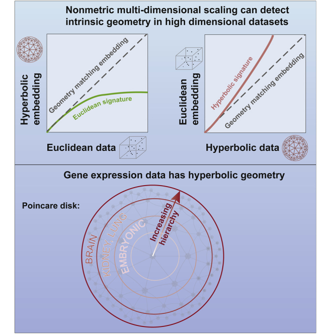
Graphical abstract
Highlights
-
•
A method to identify underlying low-dimensional geometry in high-dimensional dataset
-
•
Gene expression data exhibit local Euclidean and large-scale hyperbolic geometry
-
•
The size of the hyperbolic map is larger in differentiated and brain cells
-
•
Taking into account hyperbolic geometry yields improved visualization of data
Genes; Cell Biology; Complex Systems
Introduction
One of the great challenges of modern biology is to understand how the genotype of an organism impacts its phenotype, such as disease risk. The difficulty of this problem stems from the complexity of this relationship where thousands of genes can affect a phenotype of interest through nonlinear interactions (The Wellcome Trust Case Control Consortium, 2007; Manolio et al., 2009; Yang et al., 2010). In the past 15 years, genome-wide association studies have demonstrated that a range of traits, including those that are related to metabolic and mental health disorders, are potentially linked to thousands of genes, with each gene explaining only a small fraction of the expected heritability (Manolio et al., 2009). At the same time, correlations between genes are widespread (Novembre et al., 2008). These observations raise the possibility that genetic variation and their expression can be described by a low-dimensional geometry. Identifying this geometry would make it easier to find relevant gene combinations and how they impact a given trait.
Traditional approaches to finding low-dimensional spaces, such as the principal-component analysis (PCA), assume that the space is “flat” (i.e., has zero curvature) and evaluate distances between points according to Euclidean metric. Recently, hyperbolic spaces have attracted a lot of attention both for the analysis of biological data (Zhou et al., 2018; Klimovskaia et al., 2020; Ding and Regev, 2019) and in computer science (Wilson et al., 2014; Nickel and Kiela, 2017; Walter and Ritter, 2002; Shavitt and Tankel, 2008; Cvetkovski and Crovella, 2017; Ovinnikov, 2019; Ganea et al., 2018). The reason for this interest is that hyperbolic metric approximates the exponential expansion of possible states of the system described by a hierarchical tree-like process (Krioukov et al., 2010). Hierarchical representations, such as phylogenetic trees and clustering clades have long been used to characterize differences between cells (Eisen et al., 1998), proteins (Manning et al., 2002), the activity of metabolic networks within cells (Ravasz et al., 2002; Dunkel et al., 2014), and human brain functional networks (Meunier et al., 2009). This suggests that hyperbolic metric should be considered as one of the possibilities when searching for the low-dimensional geometry in biological data. At the same time, any hyperbolic geometry (which has negative curvature) can locally be approximated using Euclidean geometry (which has zero curvature). Therefore, in this work we focus on comparing the signatures of Euclidean and hyperbolic geometry. For completeness, we also include results from the spherical geometry that has positive curvature and represents the remaining of three possible geometries with constant curvature.
In this work we pursue two goals. The first goal is to develop a quantitative test for distinguishing the curvature of the underlying low-dimensional geometry. We show that this can be achieved by performing non-metric multi-dimensional scaling using both Euclidean and hyperbolic metric and comparing the results. Our second goal is to develop visualization tools for data that exhibit a low-dimensional hyperbolic geometry. Many of the current state-of-the-art visualization tools, such as k-means clustering (MacQueen, 1967), local linear embedding (Roweis and Saul, 2000), t-distributed Stochastic Neighbor Embedding (t-SNE) (Maaten and Hinton, 2008; Zhou and Sharpee, 2018), and Uniform Manifold Approximation and Projection (UMAP) (Becht et al., 2019), all use Euclidean metric. We propose a method for incorporating hyperbolic metric into the t-SNE method and show that this leads to improved visualization across a range of datasets.
To demonstrate the utility of both the diagnostic method and the hyperbolic t-SNE (h-SNE), we apply these methods to a range of gene expression datasets from mouse and human. These datasets uniformly show that gene expression data across different cell types exhibit a low-dimensional hyperbolic geometry. The curvature of this space, which is related to the branching ratio of the corresponding tree-like process, was systematically higher in differentiated cell types compared with embryonic cells and took even larger values for brain cells. These results demonstrate that gene expression data can be effectively described using a small number of coordinates under hyperbolic metric. Visualizations using hyperbolic metric consistently showed more accurate representations, both in terms of local and large-scale structure, including more consistent estimates of developmental states in datasets where pseudo-time trajectories could be constructed (Klimovskaia et al., 2020).
Results
Non-metric MDS outperforms metric MDS in geometry detection
Multi-dimensional scaling (MDS) has been widely used to embed a set of data points into a geometric space in a way that attempts to best preserve the distances between points in the original space. Metric MDS tries to make the embedding distances proportional to the input distances, whereas non-metric MDS only preserves the ordinal values, allowing a monotonic nonlinear transformation between the distances. Both metric and non-metric MDS in high-dimensional Euclidean space have been well studied during the past few decades. However, the MDS in the hyperbolic space has not been fully developed yet. Several metric MDS algorithms have been proposed recently for embedding data into hyperbolic space, offering advantages over Euclidean visualizations in terms of distance preservation, space capacity, trajectory inference, and unseen data prediction (Sala et al., 2018; Klimovskaia et al., 2020; Wilson et al., 2014; Nickel and Kiela, 2017; Walter and Ritter, 2002; Shavitt and Tankel, 2008; Cvetkovski and Crovella, 2017; Ovinnikov, 2019; Ganea et al., 2018; Ding and Regev, 2019), etc. However, we find that metric MDS does not correctly distinguish between Euclidean and hyperbolic geometry of input data, but non-metric MDS does (Figure 1). The reason for this is that non-metric MDS matches the ranking order instead of exact values of the data distances. The resulting nonlinear distortions in embedding distances can be used as indicators for a geometry mismatch between data and embedding points. When using non-metric MDS, we illustrate that as soon as there is a mismatch between native and embedding geometry, a nonlinear distortion appears in the scatterplots of embedding distances versus input data distances (Figures 1A and 1B). These scatterplots are known as Shepard diagrams (Shepard, 1980). When Euclidean data are embedded into a hyperbolic space, the Shepard diagram has negative convexity (Figure 1A). When hyperbolic data are embedded into Euclidean space, the Shepard diagram has a positive convexity (Figure 1B). Thus the convexity of the Shepard diagram can indicate the difference in geometric properties between the embedding and native spaces, and in particular could indicate the difference in curvature of geometry. When using the metric MDS, the Shepard diagram shows increased spread (Figure 1D) but does not yield a nonlinear relationship upon embedding Euclidean data to hyperbolic space (Figure 1C). The reason is that Euclidean distances can be fully embedded into the faster-expanding hyperbolic space masking the distortion of distances, and this does not happen in the non-metric MDS (Shepard, 1980). In what follows we apply non-metric MDS to synthetic and several real gene expression datasets to detect their hidden geometry, and we refer to non-metric MDS as simply MDS for brevity.
Figure 1.

Shepard diagrams for metric MDS and non-metric MDS applied to synthetic geometric data with either Euclidean or hyperbolic native geometry
(A–D) These simulations were produced by (1) randomly sampling 100 points in 5D Euclidean (A and C) and hyperbolic space (B and D), (2) computing geometric distances using the corresponding distance metrics, and (3) using either non-metric MDS (A and B) or metric MDS (C and D) to embed the points to 5D Euclidean and hyperbolic space. The radius of the hyperbolic space (measured in units of inverse curvature) was 3.0 for both the sampling and embedding spaces. The convexity of Shepard diagrams reflects the difference in geometry between the embedding and native spaces; it is positive when hyperbolic data are embedded in Euclidean space and negative when Euclidean data are embedded into the hyperbolic space. These differences are less distinct in the case of metric MDS (bottom row).
Synthetic geometric data
When cells are characterized according to the expression of thousands of genes, the number of genes represents the nominal dimension of the representation space. However, the real dimension of the gene expression space might be much lower. Furthermore, the true geometry of the hidden space is not necessarily Euclidean. Therefore, in this section we analyze the signatures of low-dimensional geometry of constant curvature (either Euclidean, spherical, or hyperbolic) in the situation where each data point is described with respect to large number of variables. In the synthetic examples below, the points are first sampled from a low-dimensional geometry and then embedded into a high-dimensional Euclidean space. This step is included to mimic analysis of experimental data, where each data point is evaluated according to a large number of measurements. After this, the data points are embedded into spaces of different curvatures to determine indicators through which the properties of the original low-dimensional space can become apparent. In the examples below, we focus primarily on hyperbolic and Euclidean geometries, because hyperbolic geometry describes hierarchically organized data, whereas Euclidean metric is often the only feasible geometric metric for computing distances of high-dimensional vectors. Comparison with the results for spherical spaces is provided in Figure S1.
First, we analyze the case where data have a 5D Euclidean underlying geometry. To simulate this case we randomly sample 100 points from a 5D Euclidean space and use Euclidean MDS (EMDS) to embed the points to 5D, 10D, 50D, and 100D space, respectively (Figure 2A, left). This step emulates the representation of real data where each data point is described by a large number of measurements (e.g., transcriptome) according to which each cell is characterized, and the distances between points are measured according to a Euclidean metric. The embeddings with different number of dimensions correspond to cases where measurements are taken with respect to different number of genes. As expected, the distances of synthetic 5D Euclidean points can be preserved without distortion when embedding data to Euclidean spaces of higher dimensions. This is evidenced by the linearity of Shepard diagrams in the left column of Figure 2A. Next, we apply EMDS (Figure 2A, middle) and hyperbolic MDS (HMDS) (Figure 2A, right) to the points in the Euclidean representation space, as we did in Figures 1A and 1B. As one can see in Figure 2A, Euclidean embeddings of these data do not generate distortions in the Shepard diagrams, but hyperbolic embeddings yield Shepard diagrams with negative convexity that is largely independent of embedding dimensions. This indicates that the data have an underlying Euclidean geometry.
Figure 2.

Illustration of the diagnostic approach based on MDS for geometry detection on synthetic data
(A) Randomly sampled 100 points from 5D Euclidean space are embedded into 5, 10, 50, and 100 dimensional Euclidean spaces (left), followed by subsequent embeddings into 5D Euclidean space (middle) or hyperbolic space (right). The solid lines represent the fits using Equation (1), the Shepard diagram curvatures κ are shown at the top of each panel.
(B) Same analysis for 100 sampled points from a 5D hyperbolic space with Rdata = 3.0. The hyperbolic radii used in HMDS are Rmodel = 3.0 in both (A) and (B).
To quantitatively characterize Shepard diagrams we fit them using:
| (Equation 1) |
where x and y represent distances of points before and after embedding, respectively; parameter x0 = min(x)−ε is the distance offset representing the difference caused by noise from biological variations or experimental measurements, with a small ε introduced to avoid zero input values in the fitting. The parameter κ is key because it characterizes the convexity of Shepard diagrams. The zero κ = 0 indicates pure linearity and an exact match between the model and data geometries, whereas κ ≠ 0 indicates convexity and a mismatch between the two geometries. So the sign of κ can indicate the difference in curvature between two spaces. In the current examples, κ = 0 in EMDS and κ = −0.5 in HMDS embedding with Rmodel = 3, with no changes as the representation dimension (Figure 2A). These values describe the signatures of data that have intrinsic Euclidean geometry (Figure 1A).
The situation is qualitatively different for the case where the data have a hidden hyperbolic geometry, cf. Figure 2B. Here we sample 100 points from a 5D hyperbolic space with Rdata = 3.0. The initial embedding of these points into a low-dimensional Euclidean space produces distortions, indicating that using Euclidean metric to evaluate hyperbolic distances between points will not be accurate when using the same dimension for the embedding space. However, Euclidean embeddings into larger dimensional spaces can produce accurate distance representations. For example, in the left column of Figure 2B, accurate distance representation is obtained starting with ∼50 embedding dimensions. The reason for this is that in a large-dimensional Euclidean space points could be distributed along hyperbolic manifolds, approximating the true hyperbolic metric. We next apply MDS to examine the geometry of the representations by embedding them into a low-dimensional Euclidean (middle column) or hyperbolic space (right column). With the increase of representation dimension, the convexity parameter κ of the Shepard diagram increases from approximately zero value (κ = −0.06) to κ = 1.05 in EMDS and increases from κ = −0.58 to an approximately zero value (κ = −0.04) in HMDS (Figure 2B). These signatures (Figure 1B) indicate that hyperbolic property is more fully preserved when points are characterized with respect to more dimensions. These analyses of synthetic data illustrate how a combination of EMDS and HMDS can be used to elucidate the intrinsic geometry starting with the initial Euclidean representation. This method can also be used to detect spherical geometry, which has positive curvature. Synthetic results show that spherical geometry has opposite property as hyperbolic geometry: spherical is to Euclidean looks like what Euclidean is to hyperbolic in Shepard diagram (Figure S1).
Geometry of gene expression data
We now apply this method to analyze the intrinsic geometry of gene expression data. We first analyze a discrete gene expression data from Lukk et al. (2010). In the article, they integrated microarray data from 5,372 human samples representing 369 different cell and tissue types, disease states, and cell lines, which has a complex global structure. They constructed a global gene expression map by performing PCA and found that the first two principal axes described variation in biological variables corresponding to hematopoietic and malignancy properties. However, the presence and properties of the underlying low-dimensional geometry and how the samples are organized in the space remain to be investigated. Several previous studies showed that gene expression was stochastic both at the single cell level and the population level (Elowitz et al., 2002; Oleksiak et al., 2002; Raj and van Oudenaarden, 2008), and the expression profiles of samples within the same cluster were dominated by intrinsic noise (Elowitz et al., 2002). This would imply either Euclidean geometry, at least locally, or a lack of geometric structure altogether. On a global scale, biological systems usually show a hierarchical structure, which would imply hyperbolic geometry (Ravasz et al., 2002; Meunier et al., 2009). Therefore, we separately probe the geometry of gene expression data at the local and global scales. To probe local geometry we apply k-means (k = 50) method to cluster the whole data and select 100 samples from a single cluster randomly. Similarly to Figure 2, we use increasing subsets of genes (from 20 probes to all the 22,283 probes) to represent samples and then perform EMDS and HMDS embeddings (Rmodel = 2.6) for geometry detection (Figure 3A). Increasing the number of probes with respect to which samples were characterized corresponds to increasing the dimensionality of the initial Euclidean embedding as in Figure 2. We find that this does not significantly change the convexity of the Shepard diagram in both EMDS and HMDS (κ ≈ 0 in EMDS and κ ≤ −0.4 in HMDS). These results match the fitting in Figure 2A and indicate that the samples taken from the same cluster have Euclidean structure, even when all the probes are used (Figure 3A). Additional analyses show that the Euclidean structure is indeed caused by the stochastic Gaussian expressions of genes among the samples within a cluster (Figure S2).
Figure 3.

Human gene expression has locally Euclidean and globally hyperbolic hidden geometry
(A) MDS embedding results for samples taken from a single k-means cluster, with distances evaluated by Euclidean metric with respect to increasing number of probes. Left and right columns show results of embeddings into 5D Euclidean and hyperbolic space, respectively.
(B) Same analysis for samples taken randomly from the whole data. The hyperbolic space used in HMDS had radius Rmodel = 2.6 in both (A) and (B).
Variations in gene expression across samples taken from different clusters, which represent different cell types, tissues, and disease states, show more complicated distributions (Figure S2) and have attracted a great deal of attention (Aguet et al., 2017). To study the geometric structure of expression space globally, we selected 100 samples randomly from the whole population instead of local clusters and performed the same embeddings as in Figure 3A. Surprisingly we find that, as the number of probes increases, the convexity of the Shepard diagram increases from being approximately zero κ = −0.07 to κ = 0.64 in EMDS and from κ = −0.42 to κ = 0.05 in HMDS (Figure 3B). These fitting results match the signatures expected for hyperbolic geometry in Figure 2B. It shows that the gene expression space has hyperbolic structure that becomes increasingly more apparent upon including a moderately large number of genes (>1,000 probes) in the measurements.
To test the robustness of this conclusion and make full use of the whole data, we repeat the sampling process 300 times both for the local sampling where samples are taken from different single clusters and for the global sampling where samples are broadly taken from the whole data. The samples are taken with replacement. As expected, for samples taken from local clusters, the median values of convexity κ ≈ 0 in EMDS and κ < 0 in HMDS (Figures 4A and 4B) even when all genes are used. These measurements indicate Euclidean structure. For samples taken across the whole population, with increasing number of probes, the median of κ increases to be positive in EMDS and close to zero in HMDS (Figures 4C and 4D); these signatures indicate that samples across population have hyperbolic structure when represented by a moderately large number of genes (≥1,000 probes).
Figure 4.

Statistics of convexity parameter of Shepard diagrams across human gene expression data
(A and B) Violin plots show the convexity statistics in 5D EMDS (A) and 5D HMDS (B) across 300 repeated samplings from different k-means clusters, as a function of the number of probes. 100 data points are taken in each sampling.
(C and D) Same analysis for samples taken with replacement from the whole data. The black dashed lines show κ = 0 and signify Euclidean geometry in EMDS (A and C) or hyperbolic geometry with Rdata = Rmodel = 2.6 in 5D HMDS (B and D). In each plot, the width of the shape shows the probability density of different values; the central line, the left edge and right edge of the box within the shape represent the median, the 75th, and the 25th percentiles respectively. The line within the shape extends to the most extreme non-outlier points; the outliers are represented by dots.
The size of the hyperbolic gene expression map varies systematically across cell types
The HMDS method can also be used to estimate the curvature of the underlying low-dimensional space or equivalently the size of the hyperbolic map measured in units of inverse curvature (Figure S3). The hyperbolic radius Rdata can be used as an indication of the hierarchical depth of the corresponding tree structure (Krioukov et al., 2010). Above we have shown that global human gene expression data can be embedded without distortion to 5D hyperbolic space with Rmodel = 2.6. This value was obtained by systematically screening across different R values to find those best matching Rdata as indicated by the zero convexity parameter κ obtained by fitting the corresponding Shepard diagram. In Figure 5A we show that the convexity κ decreases with Rmodel and crosses 0 at Rmodel≈2.6. Therefore, we conclude that Rdata = 2.6 in 5D hyperbolic representation. Next, we examine several other gene expression datasets and determine Rdata for them. Han et al. (2018) performed Microwell-seq of cells from multiple mouse organs and generated mouse cell atlas map using the t-SNE method. Here we re-analyze these data to find if they have a nonlinear low-dimensional structure. The microwell-seq data in this dataset are much sparser than the microarray data. Therefore, we first check whether changes in sparseness of measurement data could affect the geometry detection and its parameters. To this end, we re-analyze synthetic data where at the stage of Euclidean high-dimensional embedding all values are re-set to zero if their values are in the smallest 5%. Even though intermediate embeddings into larger dimensional space have more values that are set to zero, this does not change the estimated convexity values for low-dimensional embeddings using either Euclidean or hyperbolic metric, and the tests correctly identify the presence of a low-dimensional hyperbolic geometry (Figure S4).
Figure 5.

Radius of the hyperbolic space of gene expression varies systematically across cell types
(A–E) The violin plots of convexity of Shepard diagrams κ as a function of the radius of the embedding space Rmodel. (A) Microarray data from human samples in Lukk et al. (2010) dataset. (B–E) Microwell-seq data (Han et al., 2018) for brain cells (B), kidney (C), lung (D), and embryonic stem cells (E). Solid lines show the linear regression; their y-intercepts yield estimates of the radius of the hyperbolic map for each dataset (see printed values with ±2 SD from 300 samplings). The HMDS embedding dimension is D = 5 in (A–E).
(F) Dependence of the radius of the hyperbolic space as a function of the embedding dimension for datasets in (A–E) on human cells (HS), mouse brain (MB), mouse kidney (MK), mouse lung (ML), and mouse embryonic cells (ME). Rdata = 0 (D ≥ 8 in ME) means that κ remains negative regardless of Rmodel.
With these checks at hand, we proceeded to analyze the microwell-seq data from different mouse organs. Following previous studies (Macosko et al., 2015), the data were pre-processed using the Seurat algorithm (Butler et al., 2018) and projected onto top 50 principal components (see transparent methods). Next, we applied 5D HMDS to the processed data from four of the mouse organs – brain, kidney, lung, and embryonic stem cells. We find that all these data have an underlying hyperbolic structure (Figures 5B–5E). It is worth noting that the hyperbolic radius necessary to describe these data is smaller than that for human samples. Among the four mouse cell types, the largest radius is found for the mouse brain cells with Rbrain = 2.03 ± 0.02 (Figure 5B), followed by mouse kidney and lung that have similar radii Rdata = 1.78 ± 0.02 and 1.77 ± 0.02, respectively (Figures 5B and 5C). Finally, the smallest radius is observed for mouse embryonic stem cells with Rdata = 1.15 ± 0.04 (Figure 5E). Because hyperbolic radius indicates the depth of the underlying hierarchical tree, these findings indicate an interesting progression in complexity with embryonic cells exhibiting the smallest degree of hierarchical organization and brain cells exhibiting the largest degree.
We note that the HMDS methods produce estimates of the hyperbolic radius that depend on the embedding dimension D. This happens because the density of points increases exponentially with exponent (D−1)R according to Equation (S3). Results in Figures 5A–5E are obtained for a 5D hyperbolic space. In panel F, we show how the estimates of Rdata decrease with embedding dimension in different datasets (Figure 5F). Importantly, the relative differences in Rdata across cell types are maintained across a range of different embedding dimensions. The hyperbolic maps continue to have the smallest radius for mouse embryonic cells, larger values for mouse differentiated cells, and yet larger values for mouse brain and human cells. We also find that the minimal embedding dimension for all of these datasets is D = 3, and that smaller dimension fails to properly embed the data.
We also tested the robustness of the HMDS method to noise in the data. Toward that goal, we add varying amounts of the multiplicative Gaussian noise to the Lukk et al. data (Lukk et al., 2010) and fit the resulting Shepard diagrams. The fits produce stable convexity estimates for Shepard's diagrams over a broad range of noise values (Figures S5A–S5E). This robustness is observed up to very large noise values with ε = 0.5 when noise completely destroys the data structure (Figure S5F). The reason for this robustness is that noise does not systematically shift the shape of the Shepard diagram, yielding the same fitting exponent under varying noise amounts.
Hyperbolic low-dimensional visualization of gene expression data
Although MDS embedding can be used to detect intrinsic geometry, it is not ideal for low-dimensional visualization. One of the primary reasons common to all MDS-based algorithms is that they are not designed to attract similar points together like t-SNE. Consequently, MDS-based methods achieve poor clustering results. These limitations were solved by nonlinear methods like t-SNE and UMAP, which, however, are only performed in the Euclidean space. As a result, existing visualization methods may cause distortion of global structure in the data that has a global hyperbolic structure. Here we aim to adapt the t-SNE algorithm to work in hyperbolic space. To achieve this we use hyperbolic metric to evaluate global distances in the data while keeping the local clustering aspects of the algorithm. The standard t-SNE method effectively discards large distance information between distant points. We recently proposed a variant of t-SNE, which aims to preserve global Euclidean structure in the data, which was called global t-SNE (g-SNE) (Zhou and Sharpee, 2018). The g-SNE method works by adding to the similarity distance measures present in the t-SNE another term that focuses on large Euclidean distances (see transparent methods). When applied to Lukk et al. data (Lukk et al., 2010), g-SNE preserves data distances very well (Figure 6A, R = 0.848). Despite the high quality of embedding, g-SNE cannot reveal the hierarchical structure of data, which is only visible in hyperbolic embedding. Therefore, considering that human gene expression space is locally Euclidean and globally hyperbolic, we develop a hyperbolic t-SNE (h-SNE) method that applies hyperbolic metric to global similarities as defined in g-SNE (Zhou and Sharpee, 2018) while still using Euclidean metric for original local similarities. We find that h-SNE gives similar embedding accuracy as g-SNE, both of which largely outperform PCA and UMAP, with R = 0.841 for h-SNE compared with R = 0.744 for PCA and R = 0.627 for UMAP (Figure 6A). The distance correlation of Shepard diagram generally quantifies the quality of embedding with respect to large distances, i.e., the global inter-class structure preservation. To measure the local structure preservation, we use the silhouette score, which measures the quality of clustering (Rousseeuw, 1987). Here we find that h-SNE achieves higher silhouette score than g-SNE and significantly higher score than other algorithms (Figure 6B).
Figure 6.

Comparison of two-dimensional visualizations of human expression data (Lukk et al., 2010) using g-SNE, h-SNE, PCA, and UMAP
(A) Shepard diagrams of the four different mappings. The Pearson correlation coefficients of pairwise distances plots are shown at the top of each panel. The shaded regions represent the 95% range of the points at each of the binned data distance intervals (20 bins), the lines in the middle represent the medium.
(B) Quantification of local and global structure preservation using Pearson correlation coefficient of Shepard diagram (y axis) and Silhouette score (x axis), respectively, for five algorithms (including t-SNE). The Silhouette score is defined as the geometric mean of the three scores obtained by using six hematopoietic labels, four malignancy labels, and fifteen subtype labels, respectively (see transparent methods).
(C) In h-SNE, the data points are visualized within a 2D Poincaré disk with order-7 triangular tiling, which represents a compressed version of a hyperbolic space. In g-SNE, PCA, and UMAP, the points are visualized in 2D Euclidean plane. Four cell types are highlighted with color: nervous system neoplasm (cyan), breast cancer (magenta), solid tissue neoplasm cell line (green), and non-neoplastic cell line (yellow). The rest of the data points are shown in gray to avoid confusion between multiple colors; see Figure S6 for colors across all cell types.
(D) The embedding samples are colored using subtractive CMY color mode according to normalized expressions of three marker genes NCAM1 (nervous system neoplasm), ASPN (breast cancer), and PLOD2 (non-neoplastic cell line).
See also Figure S6.
These quantitative improvements by h-SNE are also reflected in the improved local and global visualizations that the method provides. For local visualization, the clusters identified by h-SNE are well separated with respect to 15 different tissues and disease types (Figure S6). By comparison, the PCA representation does not separate the 15 clusters very well, mixing nervous system neoplasm cells (cyan) with the breast cancer cells (magenta) (Figure 6C). The non-neoplastic cell line (yellow) is also not separated in the PCA representation from the solid tissue neoplasm cell line (green) (Figure 6C, see all the 15 labels in Figure S6). The UMAP methods separate clusters better but generate too many disconnected components that are difficult to be matched to sample labels (Figure S6). In terms of global properties, the h-SNE visualization generates a clearer global hierarchical organization of clusters, which is not attainable in g-SNE embedding: cells from nervous system neoplasm, breast cancer, non-neoplastic cell line, and solid tissue neoplasm cell line are sequentially positioned at different branches in the disk (Figure 6C); in addition, the two principal hematopoietic and malignancy axes can be clearly identified in h-SNE, but not in UMAP (Figure S7). Finally, it is particularly interesting to note the differences in hierarchical positioning that are assigned to breast cancer cells (magenta). Many of these cells occupy points with smaller radii. Positions that are closer to the center of the hyperbolic space typically correspond to more de-differentiated cells, as we have already seen in the comparison between mouse embryonic cells and differentiated cells. Thus, the more central positions assigned to breast cancer cells are consistent with observations of them being close to de-differentiated cells (Friedmann-Morvinski and Verma, 2014).
The quality of h-SNE visualization is also illustrated by the topography with respect to gradient expressions of three marker genes: NCAM1 (Deborde et al., 2016) for nervous system neoplasm, ASPN (Castellana et al., 2012) for breast cancer, and PLOD2 (Song et al., 2017) for non-neoplastic cell line. These marker genes are highly expressed in distinct but continuous branches in h-SNE; by comparison, the expression patterns of these three genes are more difficult to organize in g-SNE, to cluster in UMAP, or to separate in PCA (Figure 6D).
In addition to visualizing discrete data, hyperbolic embedding is especially useful in representing temporally continuous data and predicting lineage information. Klimovskaia et al. (2020) developed Poincaré map method to visualize hierarchies in single-cell data. This method used similar idea as t-SNE but implemented hyperbolic metric in the representation space. This has led to improvements in the representations of cell trajectories. However, the Poincaré map method, being based on t-SNE, still largely discards large distance information. This problem can be well solved by h-SNE, which is designed to capture global hyperbolic structure. For comparison with the Poincaré map method (Figure 4 in Klimovskaia et al., 2020), we select the mouse hematopoiesis data in Moignard et al. (2015). This dataset consists of cells from different development stages: primitive streak (PS), neural plate (NP), head fold (HF), four somite GFP (Runx1) negative (4SG-), and four somite GFP positive (4SG+). We first apply HMDS method to determine the intrinsic geometry of the data and find that the data space is hyperbolic with Rdata = 1.72 (Figure S8). Then we apply h-SNE to the data and compare the results with Poincaré map. The h-SNE method produces similar local clustering as in Poincaré map, but it generates very distinct global pattern: the two differentiated branches 4SFG and 4SG extend around the disk with clear division along the angular variable in the h-SNE visualization (Figure 7A). The corresponding pattern is not as clear in Poincaré map (Figure 7B). The Shepard diagrams of the embeddings show that h-SNE preserves data distances much better than Poincaré map, especially the large distances (Figures 7C and 7D). When predicting the pseudo time, the h-SNE method produces a clear pseudo time prediction with a much smaller variance compared with the Poincaré map (c.f. compare the pseudo time in 4SFG stage, Figures 7E and 7F). Finally, as another example, we show the normalized gene expressions of two marker genes Gfi1b (hemogenic marker) and Cdh5 (endothelial marker), finding that these two genes are differentially expressed in different branches in h-SNE (Figure 7G). This separation is not obvious in Poincaré map (Figure 7H). The clear hierarchical organization of cells in h-SNE map may help us better understand the relationships between cells at different stages.
Figure 7.

Comparison of hyperbolic embedding of mouse hematopoiesis data using h-SNE and Poincaré map
(A and B) h-SNE and Poincaré mapping of the data after centering the root node in Poincaré disk (see transparent methods). Gray cluster represents potential outliers or “mesodermal” cells (Klimovskaia et al., 2020) (Moignard et al., 2015).
(C and D) Shepard diagram of h-SNE and Poincaré mapping. The data distances are calculated using Euclidean metric in the original data space, whereas the embedding distances are calculated using hyperbolic metric.
(E and F) Predicted pseudo time from h-SNE and Poincaré mapping; the pseudo time is defined as the hyperbolic distances between points and the root node.
(G and H) Normalized gene expressions of two main genes Gfi1b (hemogenic marker) and Cdh5 (endothelial marker) in h-SNE and Poincaré maps.
Discussion
In this article we developed a non-metric MDS in hyperbolic space and showed how it can be used to detect the hidden geometry of data starting with an initial Euclidean representation. By applying this method to several gene expression datasets, we found that gene expression data exhibit Euclidean geometry locally and hyperbolic geometry globally. The radius of the hyperbolic space differed depending on the cell types. The lowest values were observed for embryonic cells and the highest values were observed for brain cells in mouse data. Given that hyperbolic geometry is indicative of hierarchically organized data (Zhou et al., 2018; Krioukov et al., 2010), and the spanned radius represents the depth of the network hierarchy, it is perhaps intuitive that the largest value would be observed for highly differentiated and specialized brain cells and the smallest value for the embryonic cells.
The method that we used to detect the presence of hyperbolic geometry was based on non-metric MDS. One can also use methods from algebraic topology (Zhou et al., 2018; Giusti et al., 2015) for this purpose, as has been recently demonstrated for metabolic networks underlying natural odor mixtures produced by plants and animals (Zhou et al., 2018). The advantage of the topological method is that it is very sensitive to changes in the underlying geometry, including its dimensionality and hyperbolic radius. However, this method is computationally intensive and does not scale well to large datasets. In contrast, the non-metric MDS method is computationally much faster. Therefore, we recommend using it as a first step in determining whether the underlying geometry is hyperbolic or Euclidean. If hyperbolic geometry is detected, then radial position of embedding points can be used to arrange data hierarchically. We have also seen that taking into account hyperbolic geometry produces better low-dimensional visualizations, cf. Figures 6 and 7.
Accurate representation of data across scales is a very active area of research (Wu et al., 2018; Ding et al., 2018; Kobak and Berens, 2018). Special attention is being devoted to developing visualization methods that can not only cluster data in a useful way but also preserve relative positions between clusters (Zhou and Sharpee, 2018; Becht et al., 2019). In particular, preserving global data structure was one of the driving factors for the UMAP method (Becht et al., 2019). Knowing the underlying geometry helps to position clusters appropriately and robustly map them across different runs in a visualization method. For example, the t-SNE method produces random positions of the clusters across different runs of the algorithm (Wattenberg et al., 2016). This problem can in part be alleviated by additional constraints on large distances (Zhou and Sharpee, 2018). Here we find that using a combination of a hyperbolic metric for large distances and Euclidean metric for local distances offers strong improvements in this respect. It also outperforms the recent Poincaré map method that implements hyperbolic metric only for local distances (Klimovskaia et al., 2020). We notice that although h-SNE is best fit for hyperbolic data, it performs similarly as g-SNE in accuracy distances preservation. A future direction is to further optimize h-SNE algorithm.
What could be the origin of hyperbolic geometry at the large scale and Euclidean at small scale? First, any curved geometry, including hyperbolic, is locally flat, i.e., Euclidean. The scale at which non-Euclidean effects become important depends on the curvature of the space. From a biological perspective, the Euclidean aspects can arise from intrinsic noise in gene expression (Elowitz et al., 2002; Oleksiak et al., 2002; Raj and van Oudenaarden, 2008). This noise effectively smoothes the underlying hierarchical process that generates the data. We find that hyperbolic effects of human gene expression can be detected by including measurements on as few as ∼100 probes. Why do hyperbolic effects require measurements along multiple dimensions? The reason is that hyperbolic geometry is a representation of an underlying hierarchical process, which generates correlations between variables. These correlations become detectable above the noise once a sufficient number of measurements are made. As an example, one can think of leaves in a tree-like network, and how their activity becomes correlated when it is induced by turning on and off branches of the network. Intuitively, these correlations generate the outstanding branches of a hyperbola. We observe that these correlations can be detected by monitoring even a relatively small (∼100) number of probes. This makes it possible to construct a global map of genes from partial measurements, and open new ways for combining data from different experiments.
Limitations of the study
The main limitations of the study pertain to computational constraints. Currently, the hyperbolic MDS methods can reliably embed several hundred data points. Therefore, we analyze data by randomly selecting 100 points at a time. The hyperbolic t-SNE (h-SNE) presented here was developed based on the t-SNE version that performs exact embedding without any speed optimization (e.g., Barnes-Hut t-SNE). As a result, it becomes computationally expensive for large datasets and convergence starts to become problematic when the number of cells becomes too large. The current version performs well with less than ∼6,000 cells.
Resource availability
Lead contact
Tatyana Sharpee, sharpee@salk.edu.
Materials availability
The data used in this manuscript are all obtained from published papers.
Data and code availability
The data can be obtained from: Lukk et al. data: https://www.ebi.ac.uk/arrayexpress/experiments/E-MTAB-62/. Han et al. data: https://www.ncbi.nlm.nih.gov/geo/query/acc.cgi?acc=GSE108097; and Moignard et al. data: https://github.com/facebookresearch/PoincareMaps/blob/master/datasets/Moignard2015.csv. The codes for non-metric hyperbolic MDS are available from: https://github.com/gyrheart/Hyperbolic-MDS.git. The codes for hyperbolic t-SNE are available from https://github.com/gyrheart/Hyperbolic-t-SNE.git.
Methods
All methods can be found in the accompanying Transparent Methods supplemental file.
Acknowledgments
This research was supported by an AHA-Allen Initiative in Brain Health and Cognitive Impairment award made jointly through the American Heart Association and the Paul G. Allen Frontiers Group: 19PABH134610000, Dorsett Brown Foundation, Aginsky Fellowship, NSF grant IIS-1724421, NSF Next Generation Networks for Neuroscience Program (Award 2014217), and NIH grants U19NS112959 and P30AG068635.
Author contributions
Both authors participated in the design of this study and writing of the manuscript. Y.Z. analyzed the data.
Declaration of interests
The authors declare no competing interests.
Published: March 19, 2021
Footnotes
Supplemental information can be found online at https://doi.org/10.1016/j.isci.2021.102225.
Supplemental information
References
- Aguet F., Brown A.A., Castel S.J., Davis J.R., He Y., Jo B., Mohammadi P., Park Y., Parsana P., Segrè A.V., Strober B.J., Zappal Z. Genetic effects on gene expression across human tissues. Nature. 2017;550:204. doi: 10.1038/nature24277. [DOI] [PMC free article] [PubMed] [Google Scholar]
- Becht E., McInnes L., Healy J., Dutertre C.-A., Kwok I.W., Ng L.G., Ginhoux F., Newell E.W. Dimensionality reduction for visualizing single-cell data using umap. Nat. Biotechnol. 2019;37:38. doi: 10.1038/nbt.4314. [DOI] [PubMed] [Google Scholar]
- Butler A., Hoffman P., Smibert P., Papalexi E., Satija R. Integrating single-cell transcriptomic data across different conditions, technologies, and species. Nat. Biotechnol. 2018;36:411–420. doi: 10.1038/nbt.4096. [DOI] [PMC free article] [PubMed] [Google Scholar]
- Castellana B., Escuin D., Peiró G., Garcia-Valdecasas B., Vázquez T., Pons C., Pérez-Olabarria M., Barnadas A., Lerma E. Aspn and gjb2 are implicated in the mechanisms of invasion of ductal breast carcinomas. J. Cancer. 2012;3:175. doi: 10.7150/jca.4120. [DOI] [PMC free article] [PubMed] [Google Scholar]
- Cvetkovski A., Crovella M. Low-stress data embedding in the hyperbolic plane using multidimensional scaling. Appl. Math. 2017;11:5–12. [Google Scholar]
- Deborde S., Omelchenko T., Lyubchik A., Zhou Y., He S., McNamara W.F., Chernichenko N., Lee S.-Y., Barajas F., Chen C.-H. Schwann cells induce cancer cell dispersion and invasion. J. Clin. Invest. 2016;126:1538–1554. doi: 10.1172/JCI82658. [DOI] [PMC free article] [PubMed] [Google Scholar]
- Ding J., Condon A., Shah S.P. Interpretable dimensionality reduction of single cell transcriptome data with deep generative models. Nat. Commun. 2018;9:2002. doi: 10.1038/s41467-018-04368-5. [DOI] [PMC free article] [PubMed] [Google Scholar]
- Ding J., Regev A. Deep Generative Model Embedding of Single-Cell Rna-Seq Profiles on Hyperspheres and Hyperbolic Spaces. BioRxiv. 2019:853457. doi: 10.1038/s41467-021-22851-4. [DOI] [PMC free article] [PubMed] [Google Scholar]
- Dunkel A., Steinhaus M., Kotthoff M., Nowak B., Krautwurst D., Schieberle P., Hofmann T. Natures chemical signatures in human olfaction: a foodborne perspective for future biotechnology. Angew. Chem. Int. Ed. 2014;53:7124–7143. doi: 10.1002/anie.201309508. [DOI] [PubMed] [Google Scholar]
- Eisen M.B., Spellman P.T., Brown P.O., Botstein D. Cluster analysis and display of genome-wide expression patterns. Proc. Natl. Acad. Sci. U S A. 1998;95:14863–14868. doi: 10.1073/pnas.95.25.14863. [DOI] [PMC free article] [PubMed] [Google Scholar]
- Elowitz M.B., Levine A.J., Siggia E.D., Swain P.S. Stochastic gene expression in a single cell. Science. 2002;297:1183–1186. doi: 10.1126/science.1070919. [DOI] [PubMed] [Google Scholar]
- Friedmann-Morvinski D., Verma I.M. Dedifferentiation and reprogramming: origins of cancer stem cells. EMBO Rep. 2014;15:244–253. doi: 10.1002/embr.201338254. [DOI] [PMC free article] [PubMed] [Google Scholar]
- Ganea O., Bécigneul G., Hofmann T. Hyperbolic neural networks. Advances in Neural Information Processing Systems. 2018:5345–5355. [Google Scholar]
- Giusti C., Pastalkova E., Curto C., Itskov V. Clique topology reveals intrinsic geometric structure in neural correlations. Proc. Natl. Acad. Sci. U S A. 2015;112:13455–13460. doi: 10.1073/pnas.1506407112. [DOI] [PMC free article] [PubMed] [Google Scholar]
- Han X., Wang R., Zhou Y., Fei L., Sun H., Lai S., Saadatpour A., Zhou Z., Chen H., Ye F. Mapping the mouse cell atlas by microwell-seq. Cell. 2018;172:1091–1107. doi: 10.1016/j.cell.2018.02.001. [DOI] [PubMed] [Google Scholar]
- Klimovskaia A., Lopez-Paz D., Bottou L., Nickel M. Poincaré maps for analyzing complex hierarchies in single-cell data. Nat. Commun. 2020;11:2966. doi: 10.1038/s41467-020-16822-4. [DOI] [PMC free article] [PubMed] [Google Scholar]
- Kobak D., Berens P. The Art of Using T-Sne for Single-Cell Transcriptomics. bioRxiv. 2018:453449. doi: 10.1038/s41467-019-13056-x. [DOI] [PMC free article] [PubMed] [Google Scholar]
- Krioukov D., Papadopoulos F., Kitsak M., Vahdat A., Boguná M. Hyperbolic geometry of complex networks. Phys. Rev. E. 2010;82:036106. doi: 10.1103/PhysRevE.82.036106. [DOI] [PubMed] [Google Scholar]
- Lukk M., Kapushesky M., Nikkilä J., Parkinson H., Goncalves A., Huber W., Ukkonen E., Brazma A. A global map of human gene expression. Nat. Biotechnol. 2010;28:322. doi: 10.1038/nbt0410-322. [DOI] [PMC free article] [PubMed] [Google Scholar]
- Maaten L.v. d., Hinton G. Visualizing data using t-sne. J. Machine Learn. Res. 2008;9:2579–2605. [Google Scholar]
- Macosko E.Z., Anindita Basu A., Satija R., Nemesh J., Shekhar K., Goldman M., Tirosh I., Bialas A.R., Kamitaki N., Martersteck E.M. Highly parallel genome-wide expression profiling of individual cells using nanoliter droplets. Cell. 2015;116:1202–1214. doi: 10.1016/j.cell.2015.05.002. [DOI] [PMC free article] [PubMed] [Google Scholar]
- MacQueen J. Some methods for classification and analysis of multivariate observations. Proceedings of the Fifth Berkeley Symposium on Mathematical Statistics and Probability. 1967;1:281–297. [Google Scholar]
- Manning G., Whyte D.B., Martinez R., Hunter T., Sudarsanam S. The protein kinase complement of the human genome. Science. 2002;298:1912–1934. doi: 10.1126/science.1075762. [DOI] [PubMed] [Google Scholar]
- Manolio T.A., Collins F.S., Cox N.J., Goldstein D.B., Hindorff L.A., Hunter D.J., McCarthy M.I., Ramos E.M., Cardon L.R., Chakravarti A. Finding the missing heritability of complex diseases. Nature. 2009;461:747–753. doi: 10.1038/nature08494. [DOI] [PMC free article] [PubMed] [Google Scholar]
- Meunier D., Lambiotte R., Fornito A., Ersche K., Bullmore E.T. Hierarchical modularity in human brain functional networks. Front. Neuroinform. 2009;3:37. doi: 10.3389/neuro.11.037.2009. [DOI] [PMC free article] [PubMed] [Google Scholar]
- Moignard V., Woodhouse S., Haghverdi L., Lilly A.J., Tanaka Y., Wilkinson A.C., Buettner F., Macaulay I.C., Jawaid W., Diamanti E. Decoding the regulatory network of early blood development from single-cell gene expression measurements. Nat. Biotechnol. 2015;33:269–276. doi: 10.1038/nbt.3154. [DOI] [PMC free article] [PubMed] [Google Scholar]
- Nickel M., Kiela D. Advances in Neural Information Processing Systems. 2017. Poincaré embeddings for learning hierarchical representations; pp. 6338–6347. [Google Scholar]
- Novembre J., Johnson T., Bryc K., Kutalik Z., Boyko A.R., Auton A., Indap A., King K.S., Bergmann S., Nelson M.R. Genes mirror geography within europe. Nature. 2008;456:98–101. doi: 10.1038/nature07331. [DOI] [PMC free article] [PubMed] [Google Scholar]
- Oleksiak M.F., Churchill G.A., Crawford D.L. Variation in gene expression within and among natural populations. Nat. Genet. 2002;32:261. doi: 10.1038/ng983. [DOI] [PubMed] [Google Scholar]
- Ovinnikov I. Poincar’e wasserstein autoencoder. arXiv. 2019 arXiv:1901.01427. [Google Scholar]
- Raj A., van Oudenaarden A. Nature, nurture, or chance: stochastic gene expression and its consequences. Cell. 2008;135:216–226. doi: 10.1016/j.cell.2008.09.050. [DOI] [PMC free article] [PubMed] [Google Scholar]
- Ravasz E., Somera A.L., Mongru D.A., Oltvai Z.N., Barabási A.-L. Hierarchical organization of modularity in metabolic networks. Science. 2002;297:1551–1555. doi: 10.1126/science.1073374. [DOI] [PubMed] [Google Scholar]
- Rousseeuw P.J. Silhouettes: a graphical aid to the interpretation and validation of cluster analysis. J. Comput. Appl. Math. 1987;20:53–65. [Google Scholar]
- Roweis S.T., Saul L.K. Nonlinear dimensionality reduction by locally linear embedding. Science. 2000;290:2323–2326. doi: 10.1126/science.290.5500.2323. [DOI] [PubMed] [Google Scholar]
- Sala F., de Sa C., Gu A., Ré C. International Conference on Machine Learning. 2018. Representation tradeoffs for hyperbolic embeddings; pp. 4457–4466. [PMC free article] [PubMed] [Google Scholar]
- Shavitt Y., Tankel T. Hyperbolic embedding of internet graph for distance estimation and overlay construction. IEEE/ACM Trans. Networking (Ton) 2008;16:25–36. [Google Scholar]
- Shepard R.N. Multidimensional scaling, tree-fitting, and clustering. Science. 1980;210:390–398. doi: 10.1126/science.210.4468.390. [DOI] [PubMed] [Google Scholar]
- Song Y., Zheng S., Wang J., Long H., Fang L., Wang G., Li Z., Que T., Liu Y., Li Y. Hypoxia-induced plod2 promotes proliferation, migration and invasion via pi3k/akt signaling in glioma. Oncotarget. 2017;8:41947. doi: 10.18632/oncotarget.16710. [DOI] [PMC free article] [PubMed] [Google Scholar]
- The Wellcome Trust Case Control Consortium Genome-wide association study of 14,000 cases of seven common diseases and 3,000 shared controls. Nature. 2007;447:661. doi: 10.1038/nature05911. [DOI] [PMC free article] [PubMed] [Google Scholar]
- Walter J.A., Ritter H. Proceedings of the Eighth ACM SIGKDD International Conference on Knowledge Discovery and Data Mining. ACM; 2002. On interactive visualization of high-dimensional data using the hyperbolic plane; pp. 123–132. [Google Scholar]
- Wattenberg M., Viégas F., Johnson I. How to use t-sne effectively. Distill. 2016;1:e2. [Google Scholar]
- Wilson R.C., Hancock E.R., Pekalska E., Duin R.P. Spherical and hyperbolic embeddings of data. IEEE Trans. Pattern Anal. Mach. Intell. 2014;36:2255–2269. doi: 10.1109/TPAMI.2014.2316836. [DOI] [PubMed] [Google Scholar]
- Wu Y., Tamayo P., Zhang K. Visualizing and interpreting single-cell gene expression datasets with similarity weighted nonnegative embedding. Cell Syst. 2018;7:656–666. doi: 10.1016/j.cels.2018.10.015. [DOI] [PMC free article] [PubMed] [Google Scholar]
- Yang J., Visscher P.M., Wray N.R. Sporadic cases are the norm for complex disease. Eur. J. Hum. Genet. 2010;18:1039–1043. doi: 10.1038/ejhg.2009.177. [DOI] [PMC free article] [PubMed] [Google Scholar]
- Zhou Y., Sharpee T. Using Global T-Sne to Preserve Inter-cluster Data Structure. bioRxiv. 2018:331611. [Google Scholar]
- Zhou Y., Smith B.H., Sharpee T.O. Hyperbolic geometry of the olfactory space. Sci. Adv. 2018;4:eaaq1458. doi: 10.1126/sciadv.aaq1458. [DOI] [PMC free article] [PubMed] [Google Scholar]
Associated Data
This section collects any data citations, data availability statements, or supplementary materials included in this article.
Supplementary Materials
Data Availability Statement
The data can be obtained from: Lukk et al. data: https://www.ebi.ac.uk/arrayexpress/experiments/E-MTAB-62/. Han et al. data: https://www.ncbi.nlm.nih.gov/geo/query/acc.cgi?acc=GSE108097; and Moignard et al. data: https://github.com/facebookresearch/PoincareMaps/blob/master/datasets/Moignard2015.csv. The codes for non-metric hyperbolic MDS are available from: https://github.com/gyrheart/Hyperbolic-MDS.git. The codes for hyperbolic t-SNE are available from https://github.com/gyrheart/Hyperbolic-t-SNE.git.