Improved protein model quality assessment by integrating sequential and pairwise features using deep learning

Abstract

Motivation

Accurately estimating protein model quality in the absence of experimental structure is not only important for model evaluation and selection but also useful for model refinement. Progress has been steadily made by introducing new features and algorithms (especially deep neural networks), but the accuracy of quality assessment (QA) is still not very satisfactory, especially local QA on hard protein targets.

Results

We propose a new single-model-based QA method ResNetQA for both local and global quality assessment. Our method predicts model quality by integrating sequential and pairwise features using a deep neural network composed of both 1D and 2D convolutional residual neural networks (ResNet). The 2D ResNet module extracts useful information from pairwise features such as model-derived distance maps, co-evolution information, and predicted distance potential from sequences. The 1D ResNet is used to predict local (global) model quality from sequential features and pooled pairwise information generated by 2D ResNet. Tested on the CASP12 and CASP13 datasets, our experimental results show that our method greatly outperforms existing state-of-the-art methods. Our ablation studies indicate that the 2D ResNet module and pairwise features play an important role in improving model quality assessment.

Availability and implementation

https://github.com/AndersJing/ResNetQA.

Supplementary information

Supplementary data are available at Bioinformatics online.

1 Introduction

Significant progress has been made in computational protein structure prediction, especially template-free modeling (Kryshtafovych et al., 2019; Senior et al., 2020; Wang et al., 2017; Xu, 2019). To facilitate application of predicted 3D models, it is desirable to have an estimation of their local and global quality in the absence of experimental structures. Model quality assessment (QA) has also been used to assist protein model refinement (Adiyaman et al., 2019; Heo et al., 2019; Hiranuma et al., 2020; Park et al., 2019). Since CASP7 in 2006 (Cozzetto et al., 2007), many model QA methods have been developed, but the accuracy of local QA is still not very satisfactory, especially when all models under consideration are generated by an individual tool.

There are two major categories of protein model QA methods: consensus (or clustering) methods and single-model methods (Won et al., 2019). Some methods are the combination of these two. Consensus methods mainly rely on clustering or comparison of models of a protein target. They work well when one protein has many models generated by different methods, e.g. in CASPs. In the case there are very few models built by a single method for a protein (which is often true in real-world application), single-model QA methods are needed, which predicts quality of a model using only its own information (Derevyanko et al., 2018; Hurtado et al., 2018; Karasikov et al., 2019; Olechnovič et al., 2017; Uziela et al., 2017). Most single-model QA methods extract some features from a decoy model and then map the features to a quality score using statistical or machine learning methods. A variety of features have been studied such as physical features, statistical features, local structural features (secondary structure and solvent accessibility), and sequence features (amino acid sequence and sequence profile). There are also a few quasi single-model methods that estimate model quality by comparing it to a small number of reference models generated by a small set of popular tools (Jing et al., 2016; Maghrabi et al., 2017). The quality of a protein model can be measured at residue/atom level (i.e. local quality) and at model level (i.e. global quality), which are referred as local and global quality assessment, respectively (Cheng et al., 2019; Won et al., 2019). Local quality is valuable for evaluation of local structure error and model refinement, while global quality is valuable for model ranking and selection.

This article focuses on single-model-based local and global QA. Although single-model QA is challenging, recently some progress has been made by using new features and deep learning. For example, ProQ3D uses a multi-layer perceptron to predict model quality from carefully curated features (Uziela et al., 2017). ProQ4 predicts global QA by employing 1D fully convolutional neural network (CNN) and transfer learning (Hurtado et al., 2018). CNNQA applies 1D CNN to predict local and global model quality from sequential features, Rosetta energy terms and knowledge-based potentials (Hou et al., 2019). QDeep (Shuvo et al., 2020) uses an ensemble of stacked 1D CNNs to predict quality from predicted distance information and some similar sequential features used by CNNQA. These methods mainly use coarse-grained or residue-level structure representation. In contrast, 3D convolutional neural networks (Derevyanko et al., 2018; Pagès et al., 2019) or graph convolutional neural networks (Igashov et al., 2020; Sanyal et al., 2020) may represent a protein structure model at atom level and thus, encode more information, but they may not fare very well on those protein models with poor side-chain packing (Hurtado et al., 2018; Olechnovič et al., 2017) while predicting the widely used C_α-based quality metrics such as GDT-TS and TMscore. Although some methods have used predicted contact (Cao et al., 2017) and distance information (Shuvo et al., 2020), but they do not take full advantage of the predicted inter-residue distance (probability or potential) matrix which has greatly improved protein structure prediction recently (Greener et al., 2019; Senior et al., 2020; Xu, 2019; Zhu et al., 2018). For example, in order to use predicted distance information in its 1D deep model for global QA, QDeep (Shuvo et al., 2020) uses contact map similarity between the predicted and model-derived distance maps, which may result in information loss. To avoid this, we use 2D ResNet to directly extract information from predicted distance information.

We propose a new single-model QA method ResNetQA (a ResNet-based QA method) that may greatly improve protein model QA, by using a deep 2D dilated residual network (ResNet) to explicitly extract useful information from pairwise features such as model-based distance matrices, predicted inter-residue distance potentials and co-evolution information. These pairwise features may encode main structural information without introducing noise from side-chain or hydrogen atoms. Our method also uses a 1D deep ResNet to map sequential features (and pooled pairwise information derived from 2D ResNet) to local and global model quality. Further, to reduce bias introduced by a small training dataset, we train our deep model using a large set of decoy models of more than 14 000 proteins, in addition to CASP and CAMEO models. In particular, we built both template-based and template-free 3D models for ∼14 000 proteins randomly selected from the CATH dataset (Dawson et al., 2017) using our in-house structure prediction software RaptorX. Our experimental results show that our method outperforms latest single-model methods on both local and global QA in terms of many performance metrics. When trained by an extra ranking-based loss, our deep network can also rank decoys very well.

2 Materials and methods

2.1 Overview

Figure 1 shows the overall architecture of our deep network, mainly consisting of one 2D ResNet module and one 1D ResNet module. The 2D ResNet module extracts information from pairwise features of shape L*L*N₂ (where L is the sequence length and N₂ is the dimension of pairwise features), which are derived from multiple sequence alignment (MSA) of a protein and its 3D models. This module outputs a high-level 2D feature map of shape L*L*C (C is the channel size), which is then converted to two 1D feature maps of shape L*C by mean pooling along row and column, respectively, and fed into the 1D ResNet module together with the original sequential features. The output of the 1D ResNet module is used to predict local and global model quality. To predict local quality, one fully connected layer and one sigmoid layer are employed at each residue. To predict global quality, the output of the 1D ResNet module is converted to one vector of length 2 C+N₁ (N₁ is the dimension of sequential features) by mean pooling and fed into one fully connected layer and one sigmoid layer.

Fig. 1.

The overall architecture of our deep network for protein model local and global quality assessment. Meanwhile, L is the sequence length, C the channel size of the final 2D ResNet layer, N₁ the dimension of sequential features and N₂ the dimension of pairwise features

2.2 Datasets

We train and test our method using protein models from three sources: CASP, CAMEO and CATH. The CASP models were downloaded from http://predictioncenter.org/download_area/. The CAMEO (Haas et al., 2013) models are downloaded from https://www.cameo3d.org/sp/ and released between January 13, 2018 and September 14, 2019. Approximately 14 000 CATH domains (sequence identity <35%) are randomly selected from the CATH database (Dawson et al., 2017), and on average 15 template-based and template-free models are built for each domain using our in-house software RaptorX. These models are split into three datasets (training, validation and test) so that all models of one specific protein belong to only one dataset. The detailed information of our data is shown in the Supplementary Table S1.

The 3D models in CASP7-11 and CAMEO and the 3D models built for the CATH domains are used as our training data. The 3D models in CASP12 and CASP13 are used as the test data. We remove the 3D models in our training data from CAMEO and CATH if their corresponding proteins (i) share more than 25% sequence identity or have an BLAST E-value ≤ 0.001 (Altschul, 1997) with any test targets and (ii) have HHblits E-value ≤0.1 with any test targets. HHblits (Steinegger et al., 2019) is a popular tool that searches evolutionarily related proteins by matching profile hidden Markov models built from MSAs. After this filtering procedure, there are 14645 proteins in our training sets, among which ∼5% are randomly selected to form the validation set. Finally, there are 13916 proteins with 335468 decoys in the training set and 729 proteins with 18437 decoys in the validation set.

Only those CASP12 and CASP13 targets with publicly available experimental structures are used to test our method. Overall, there are 64 CASP12 targets with 9423 decoy models and 76 CASP13 targets with 11371 models in our test set. The 3D models in the CASP QA category are released in two stages. Since the decoy models in stage 1 are only used to check whether a method is a single-model method or a consensus method by comparing their predictions with those of stage 2 (Won et al., 2019), we mainly evaluate our method using the decoy models released at stage 2.

2.3 Feature extraction

From each protein sequence, we run HHblits (Remmert et al., 2012) to build its MSA by searching the uniclust30 database dated in October 2017, and then derive three types of features: sequential features, coevolution information and predicted distance potentials. Sequential features include: one-hot encoding of primary sequence (i.e. each residue is encoded as a binary vector of 21 entries indicating its amino acid type), rPosition (the relative position of a residue in a sequence calculated as i/L where i is the residue index), PSSM (position-specific scoring matrix derived from MSA), SS3 [3-state secondary structure predicted by RaptorX-Property (Wang et al., 2016)], and ACC [solvent accessibility predicted by RaptorX-Property (Wang et al., 2016)]. Coevolution information includes the output generated by CCMPred (Seemayer et al., 2014) and raw and APC-corrected mutual information (MI). Distance potentials are derived from distance distribution predicted by RaptorX-Contact (Xu, 2019) from MSA. Only C_β-C_β distance potential is used, and distance is discretized into 14 bins: <4, 4-5, 5-6, …, 14-15, 15-16, >16. From each protein model, we derive the following structural features: (i) secondary structure (SS3) and relative solvent accessibility (RSA) calculated by DSSP (Kabsch et al., 1983) from a 3D model; and (ii) distance maps of three atom pairs (C_αC_α, C_βC_β and NO) calculated from a 3D model. Supplementary Table S2 summarizes all these features.

2.4 Deep neural network architecture and training

As shown in Figure 1, our deep model mainly consists of 1D and 2D dilated residual neural networks (ResNet) (He et al., 2016). A gate block is used to connect pairwise input features to the 2D ResNet. It is composed of one 2D convolutional layer, one instance norm layer (Ulyanov et al., 2017) and one ELU (exponential linear unit) activation layer. As shown in Figure 2, one ResNet block consists of two instance norm layer, two convolutional layer, two ELU activation layer and one dropout layer. In a ResNet block, there is a shortcut connecting its input to the output of the second convolutional layer. In order to capture a broader context, a dilation ratio of two is used in a 2D convolutional layer. The 2D dilated ResNet can directly model the higher-order correlation between predicted and structure-derived pairwise features by convolution. In summary, our deep model contains one gate block, 10 2D ResNet blocks with 64 filters of size 5*5, 8 1D ResNet blocks with 180 filters of size 5. That is, in total our deep model consists of 21 2D convolutional layers and 16 1D convolutional layers and has about 2 million trainable parameters. We have also tested more ResNet blocks, but not observed significant improvement.

Fig. 2.

The detailed architecture of different blocks. (a) The gate block and 2D dilated ResNet block; (b) the 1D dilated ResNet block

A protein may not fit into the limited memory of a graphics processing unit (GPU). To deal with this, a sequence segment of length 350 (and its corresponding sequential and pairwise features) is randomly sampled when a protein has more than 350 residues. We implement our method with PyTorch (Paszke et al., 2019) and train it using the Adam optimizer with parameters: β1 = 0.9 and β2 = 0.999. We set the initial learning rate to 0.0001 and divide it by 2 every 3 epochs. One minibatch has 16 3D models. When we train our deep network by the ranking-based loss (described in the next paragraph), one minibatch has 8 pairs of 3D models and each pair has two models of the same target. We train our deep network 20 epochs and select the model with minimum loss on the validation data as our final model. The training and validation losses of ResNetQA and ResNetQA-R are shown in Supplementary Figure S1.

For local QA, our deep model predicts a residue-wise S-score defined by $\mathrm{S}\left(\mathrm{d}\right)=\frac{1}{1+{(d/d_0)}^2}\mathrm{ }$where d is the distance deviation of one C_α atom from its position in the experimental structure calculated by LGA (Zemla, 2003). Here we set d₀ to 3.8Å instead of 5.0Å to yield accurate prediction for small d. We convert predicted S-score to predicted distance error (or deviation) by the inverse function of S(d). For global QA, our deep model predicts GDT_TS (Global Distance Test Total Score). The loss of our deep model is the MSE (Mean Square Error) between predicted local (or global) quality and its ground truth. In order to generate deep models with better ranking performance, we have also trained our deep models (referred as ResNetQA-R) on the global margin ranking loss defined by $\mathrm{Loss}=\max (0,\mathrm{ }-\mathrm{y}\mathrm{*}(x_1-x_2\left)\right)$ where $x_1$ and $x_2$ are the predicted GDT_TS of two 3D models of the same target, and $\mathrm{y} = 1$ if the first 3D model has a better quality and -1 otherwise. Our deep network is trained to simultaneously predict local and global quality with equal weight. We have implemented our method so that it is very easy to train the network by other quality metrics, such as lDDT and CAD-score.

2.5 Evaluation metrics

We employ several widely used metrics (Won et al., 2019) to evaluate the performance of our method. To evaluate local QA, we use PCC, ASE and AUC. All models of a specific protein are pooled together when calculating PCC and AUC of local QA.

• PCC is the Pearson correlation coefficient between predicted local quality score S-score and its ground truth.

• ASE: ASE is the average residue-wise S-score similarity defined as $\mathrm{ASE}=1-\frac{1}{N}\sum _{i=1}^N\left|S\left(e_i\right)-S\left(d_i\right)\right|$, where N is the number of residues, S$\left(e_i\right)$ is the S-score derived from predicted distance deviation and S$\left(d_{\mathrm{i}}\right)$ is the S-score derived from the true distance deviation produced by LGA (Zemla, 2003). Following CASP, here the S-score is defined by $\mathrm{S}\left(\mathrm{d}\right)=\frac{1}{1+{(d/d_0)}^2}$ where d₀ = 5.0Å.

• AUC: The AUC (Area Under Curve) assesses how well the predicted score may distinguish accurate residues from inaccurate ones, where an accurate residue is the one with Cα atom deviates from its experimental position by no more than 3.8Å. AUC is the area under the ROC curve, which plots the TP (true positive rate) against the FP (false positive rate) in the prediction of accurate/inaccurate residues by varying the cut-off score for distinguishing accurate/inaccurate residues.

For global QA, we use PCC, Diff and Loss as metrics. Global metrics are calculated and averaged at the protein level.

• PCC: The Pearson correlation coefficient between predicted global quality scores and ground truth.

• Spearman: The Spearman rank correlation coefficient between predicted global quality scores and the ground truth.

• Kendall: The Kendall’s Tau rank correlation coefficient between predicted global quality scores and the ground truth.

• Diff: the mean absolute difference between predicted global quality and ground truth.

• Loss: The absolute quality difference between the best model predicted by a QA method and the real best model.

3 Results and discussion

3.1 Performance on CASP12 and CASP13 datasets

We compare our method with some single-model methods ranked well in CASP12 and CASP13 (Kryshtafovych et al., 2018; Won et al., 2019), e.g. ProQ3, Wang4, ProQ2, ZHOU-SPARKS-X and VoroMQA in CASP12 and ProQ4, VoroMQA-A, VoroMQA-B, ProQ3D and ProQ3 in CASP13. Their local and global quality estimations are downloaded from the CASP official website.

Table 1 lists the performances on the CASP12 and CASP13 stage 2 datasets. We also report the target-averaged Z-scores in Supplementary Table S3 based on the results of all groups who submitted quality estimations in CASP12 and CASP13. As shown in the table, our method significantly outperforms others on both datasets in terms of most evaluation metrics. On the CASP12 dataset, ProQ3 is slightly better than the other four methods on both local and global QA, while our method greatly outperforms ProQ3. When local QA is evaluated, our method ResNetQA is ∼29% better than ProQ3 in terms of PCC (0.5857 versus 0.4542), ∼15% better in terms of ASE (0.8527 versus 0.7408) and ∼7% better in terms of AUC (0.8077 versus 0.7518). When global QA is evaluated, our method is >16% better than ProQ3 in terms of PCC (0.8015 versus 0.6552), Spearman rank correlation (0.7053 versus 0.6036) and Kendall rank correlation (0.5430 versus 0.4407).

Table 1.

Performances of single-model methods on local (S-score) and global (GDT_TS) QA

Dataset	Method	Local			Global
		PCC↑	ASE↑	AUC↑	PCC↑	Spearman↑	Kendall↑	Diff↓	Loss↓
CASP12 Stage 2	ResNetQA a	0.5857	0.8527	0.8077	0.8015	0.7053	0.5430	7.04	7.19
	ResNetQA-R b	0.5855	0.8449	0.8063	0.8241	0.7245	0.5597	9.67	6.41
	ProQ3	0.4542	0.7408	0.7518	0.6553	0.6036	0.4407	11.04	6.15
	ProQ2	0.4363	0.6927	0.7434	0.6109	0.5702	0.4119	13.38	7.07
	Wang4	0.4126	0.7458	0.723	0.621	0.5605	0.4103	12.82	11.62
	VoroMQA	0.4098	0.7121	0.7254	0.607	0.5539	0.4014	16.68	8.44
	SPARKS-X	0.3873	0.7654	0.71	0.6759	0.6253	0.4637	13.69	7.79
CASP13 Stage 2	ResNetQA	0.5409	0.8350	0.7842	0.8051	0.7295	0.5647	7.82	10.17
	ResNetQA-R	0.5483	0.8233	0.7916	0.8220	0.7540	0.5890	11.04	8.07
	ProQ3D	0.4225	0.7314	0.7385	0.6544	0.6155	0.4542	10.60	8.52
	ProQ3	0.4122	0.7208	0.7455	0.5937	0.5647	0.4138	11.98	8.98
	ProQ4	0.3870	0.6100	0.7235	0.7197	0.6712	0.5184	13.71	8.71
	VoroMQA-A	0.3865	0.6708	0.7239	0.6450	0.5972	0.4396	15.48	10.95
	VoroMQA-B	0.3826	0.6709	0.7215	0.6205	0.5834	0.4280	15.68	9.95

^aThe model trained using local and global MSE loss.

^bThe model trained using local and global MSE loss plus global margin ranking loss.The bold content indicates the best performance in each category.

On the CASP13 dataset, our method has similar advantage over the others. When local QA is evaluated, ResNetQA is ∼28% better than ProQ3D in terms of PCC (0.5409 versus 0.4225) and ∼14% better in terms of ASE (0.8350 versus 0.7314). When global QA is evaluated, our method is >18% better than ProQ3D in terms of PCC (0.8051 versus 0.6544), Spearman (0.7295 versus 0.6155) and Kendall (0.5647 versus 0.4542). For the Loss metric, which evaluates the best ranked models but may be not very robust (Cheng et al., 2019), ResNetQA is not better than other leading methods. However, ResNetQA performs the best in terms of the Spearman and Kendall rank correlation coefficient. When trained by an extra ranking-based loss, our method (i.e. ResNetQA-R) achieves the best or second-best performances on the Loss metric, which shows the great potential of our method on different QA tasks.

To evaluate the performance of our method on superposition-free metrics, we compare our method with the others in terms of global lDDT, as shown in Supplementary Table S4. In addition, we trained two extra deep models of the same configuration to predict lDDT. Our results (in Supplementary Table S5) show that these deep models outperform ProQ4 in terms of both local and global lDDT.

3.2 Performance on CASP12 and CASP13 FM targets

Here, we examine the performance of our method on template-free modeling (FM) targets. Their predicted 3D models may have very different quality (Kinch et al., 2019), which makes QA challenging. One target is FM if it contains at least one FM evaluation unit by the CASP official definition (Abriata et al., 2018; Kinch et al., 2019).

As shown in Table 2 and Supplementary Table S6 (for Z-scores), all methods have worse performance than what is shown in Table 1. However, our method shows a larger advantage over the other methods. When local QA on the CASP12 FM targets is evaluated, our method is better than the 2^nd best method ProQ3 by ∼59% in terms of PCC (0.4494 versus 0.2830), by ∼28% in terms of ASE (0.8921 versus 0.6951) and by ∼12% in terms of AUC (0.7518 versus 0.6698). When global QA is evaluated, our method is >34% better than the 2^nd best method in terms of PCC (0.7210 versus 0.5381), Spearman rank correlation coefficient (0.7152 versus 0.5266) and Kendall’s Tau rank correlation coefficient (0.5455 versus 0.3761).

Table 2.

Performances of single-model methods on CASP12&13 FM targets

Dataset	Method	Local			Global
		PCC↑	ASE↑	AUC↑	PCC↑	Spearman↑	Kendall↑	Diff↓	Loss↓
CASP12 Stage 2	ResNetQA	0.4494	0.8921	0.7518	0.7010	0.7152	0.5455	5.36	5.76
	ResNetQA-R	0.4550	0.8803	0.7526	0.7402	0.7401	0.5684	9.61	5.54
	ProQ3	0.2830	0.6951	0.6698	0.5381	0.5266	0.3761	9.78	5.68
	ProQ2	0.2840	0.6193	0.6694	0.5147	0.5091	0.3621	14.93	8.06
	Wang4	0.2757	0.7281	0.6570	0.5503	0.5610	0.4077	7.42	8.73
	VoroMQA	0.2718	0.6605	0.6597	0.4887	0.4583	0.3231	9.07	9.28
	SPARKS-X	0.2532	0.7942	0.6457	0.5724	0.5911	0.4293	7.89	7.95
CASP13 Stage 2	ResNetQA	0.3931	0.8660	0.7231	0.7825	0.7615	0.5896	5.73	9.05
	ResNetQA-R	0.4021	0.8498	0.7392	0.8144	0.8045	0.6325	11.66	7.85
	ProQ3D	0.2521	0.6977	0.6751	0.5606	0.5501	0.3996	8.23	10.60
	ProQ3	0.2493	0.6816	0.6852	0.4887	0.4802	0.3452	10.89	10.69
	ProQ4	0.2380	0.4873	0.6661	0.6345	0.6287	0.4744	12.75	8.54
	VoroMQA-A	0.2295	0.5888	0.6624	0.5226	0.5303	0.3771	10.13	10.35
	VoroMQA-B	0.2266	0.5903	0.6602	0.5038	0.5126	0.3647	10.33	9.95

On the CASP13 FM targets, when local QA is evaluated, our method is better than ProQ3D by ∼56% on PCC, ∼24% on ASE and ∼7% on AUC. When global QA is evaluated, our method is better than ProQ3D by ∼40% on PCC, ∼38% on Spearman rank correlation and ∼48% on Kendall rank correlation. Moreover, ResNetQA-R (i.e. ResNetQA trained by an extra ranking-based loss) not only performs the best on Loss metric but also achieves better performance on most metrics over ResNetQA. In terms of lDDT our method has a larger advantage on the FM targets than other methods (Supplementary Tables S7 and S8).

3.3 Comparison with other deep learning methods

We compare our method with three leading single-model QA methods: ProQ4 (Hurtado et al., 2018), CNNQA (Hou et al., 2019) and QDeep (Shuvo et al., 2020). Meanwhile, ProQ4 performed very well in CASP13 and QDeep predicts only global quality. All these methods are built upon 1D CNN and thus, cannot make a very good use of pairwise features. Both ProQ4 and CNNQA use only sequential features. Although QDeep indeed uses predicted inter-residue distance information, its simple way of converting predicted distance information to sequential features is not as effective as the 2D ResNet used by our method. CNNQA and QDeep use energy potentials as features, but our method does not.

We evaluate our method on the same set of 40 CASP12 targets as QDeep and CNNQA were evaluated. We run ProQ4 locally with default parameters and convert its prediction to distance error by the S-function with d₀=5.0. As shown in Table 3, our method outperforms these three methods in terms of almost all metrics except the ‘Loss’ metric.

Table 3.

Performances of deep learning QA methods on 40 CASP12 targets

Method	Local			Global
	PCC↑	ASE↑	AUC↑	PCC↑	Spearman↑	Kendall↑	Diff↓	Loss↓
ResNetQA	0.5738	0.8545	0.8028	0.7910	0.6733	0.5154	6.79	7.73
ResNetQA-R	0.5709	0.8452	0.7987	0.8095	0.6812	0.5201	9.12	6.94
ProQ4	0.3884	0.7581	0.7085	0.6617	0.5851	0.4369	14.19	6.70
CNNQA	–	0.7814	–	0.6270	–	–	–	8.54
QDeep	–	–	–	0.7400	0.6570	0.4920	10.53	5.10

Note: The 40 CASP12 targets include target T0865 which was canceled later by CASP12. Here we still use it to be consistent with CNNQA and QDeep.

3.4 Contribution of different input features

We have trained three extra deep models by excluding (i) mutual information and coevolution information produced by CCMPred; (ii) predicted and model-derived secondary structures and solvent accessibilities; or (iii) predicted distance potentials. As a control, we trained a 1D deep model of eight 1D ResNet blocks without using any 2D ResNet blocks to predict model quality mainly from sequential features. To feed predicted distance potential to this 1D deep model, we apply mean pooling to distance potential at each residue. That is, we calculate the average of all pairwise potentials involving a specific residue and use the average (called marginalized distance potential) as an extra feature of this residue. By this way, our 1D deep model can also make use of pairwise information, although not very effectively. We also trained another 1D deep model of the same architecture with only sequential features but not the marginalized distance potential.

Figure 3 shows the PCC of these deep models on local QA. Their detailed performances are available in Supplementary Tables S9 and S10. It is not surprising that the 2D deep model built with all features performs the best. The 1D deep models with and without marginalized distance potential both perform very badly, which implies that the 2D ResNet module is very important. Compared to the deep model built with all features, the 2D deep model using co-evolution information but not predicted distance potential is about 9% worse on the CASP12 dataset and ∼11% worse on the CASP13 dataset. The 2D deep model without predicted and model-derived secondary structure and solvent accessibilities is about ∼4% worse on the CASP12 dataset and ∼2% worse on the CASP13 dataset. The 2D deep model using predicted distance but not co-evolution information is slightly worse than the deep model built with all features, because predicted distance potential already encodes most co-evolution information. Since the predicted distance are important for our method, we further examined the correlation between the predicted distance quality and the QA performance improvement. Our results (in Supplementary Figs S2 and S3) show that for most test proteins, predicted distance information indeed is helpful and the improvement is more pronounced for harder targets, which usually do not have very high quality of predicted distance. This makes sense since for easier targets, high-accuracy QA may also be obtained without predicted distance information. We have also trained our deep model by replacing the distance potential with the predicted distance probability on a small dataset (without the large CATH dataset due to lack of computing power). Our results (in Supplementary Table S11) show that there is only minor difference between these two types of information, and it is hard to tell which one performs better.

Fig. 3.

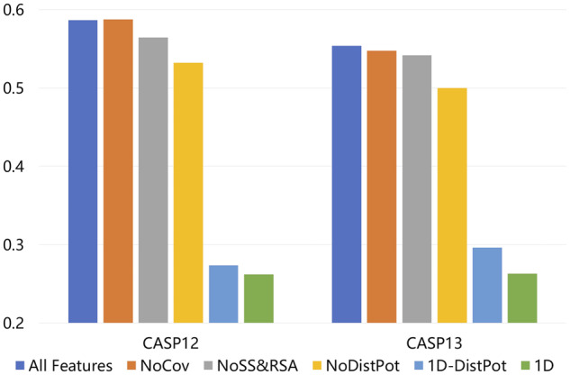
Performance (measured by PCC on local QA) of deep models built with different features. All Features: using all features. NoCov: excluding the mutual information and coevolution information produced by CCMPred. NoSS&RSA: excluding the predicted and model-derived secondary structures and solvent accessibilities. NoDistPot: excluding the predicted distance potentials. 1D-DistPot: using sequential features plus the marginalized predicted distance potentials. 1D: only using sequential features

3.5 Contribution of the CATH dataset

Many QA methods are trained by the 3D models of only hundreds of proteins in CASP and CAMEO, which have limited coverage of the whole protein universe (Bateman et al., 2017). In contrast, protein structural property prediction models (Wang et al., 2016) and contact/distance prediction models (Senior et al., 2020; Xu, 2019) usually are trained by thousands and even tens of thousands proteins. To reduce bias incurred by a small number of training proteins and improve generalization capability, we built both template-based and template-free models for about 14 000 proteins randomly selected from the CATH dataset (Dawson et al., 2017) using our in-house structure prediction software RaptorX and use these models as training data. Here we compare the performance of two deep models with exactly the same architecture and the same input features, but trained by different data. One is trained using all models built on the CASP, CAMEO and CATH datasets and the other is trained using only the CASP and CAMEO models.

Figure 4 shows a head-to-head comparison of these two deep models in terms of PCC on local QA. Their detailed performance is available in Supplementary Table S11. It is clear that the deep model trained by all 3D models works much better. On the CASP12 dataset, the deep model trained using all 3D models outperforms that trained without the CATH data by about 7.6% (0.5866 versus 0.5450). On the CASP13 data, the advantage is about 5.0% (0.5539 versus 0.5276). The result suggests that the decoy models built for CATH data is valuable for improving protein model quality assessment.

Fig. 4.

Head-to-head performance (measured by PCC on local QA) comparison of the two deep models trained with and without the CATH data. (a) CASP 12 Stage 2; (b) CASP 13 Stage 2

4 Conclusion

In this article, we have presented a new single-model QA method ResNetQA for both local and global protein model quality estimation. Our method predicts model quality by integrating a variety of sequential and pairwise features using a deep network composed of both 1D and 2D ResNet blocks. The 2D ResNet blocks extract useful information from pairwise features and the 1D ResNet blocks predict quality from sequential features and pairwise information produced by the 2D ResNet module. Our method differs from existing ones mainly by the 2D ResNet module and a larger training set. Our test results on the CASP12 and CASP13 datasets show that our method significantly outperforms existing state-of-the-art methods, especially on hard targets. In addition, our deep network can yield better ranking performance when trained by an extra ranking-based loss. Our ablation studies confirm that the 2D ResNet module and pairwise features are very important for the superior performance of our method.

Funding

This work was supported by National Institutes of Health [R01GM089753 to J.X.] and National Science Foundation [DBI1564955 to J.X.]. The funders had no role in study design, data collection and analysis, decision to publish or preparation of the manuscript.

Conflict of Interest: none declared.

References

- Abriata L.A. et al. (2018) Definition and classification of evaluation units for tertiary structure prediction in CASP12 facilitated through semi-automated metrics. Proteins Struct. Funct. Bioinf., 86, 16–26. [DOI] [PubMed] [Google Scholar]
- Adiyaman R. et al. (2019) Methods for the refinement of protein structure 3D models. Int. J. Mol. Sci., 20, 2301. [DOI] [PMC free article] [PubMed] [Google Scholar]
- Altschul S.F. (1997) Gapped BLAST and PSI-BLAST: a new generation of protein database search programs. Nucleic Acids Res., 25, 3389–3402. [DOI] [PMC free article] [PubMed] [Google Scholar]
- Bateman A. et al. (2017) UniProt: the universal protein knowledgebase. Nucleic Acids Res., 45, D158–D169. [DOI] [PMC free article] [PubMed] [Google Scholar]
- Cao R. et al. (2017) QAcon: single model quality assessment using protein structural and contact information with machine learning techniques. Bioinformatics, 33, 586–588. [DOI] [PMC free article] [PubMed] [Google Scholar]
- Cheng J. et al. (2019) Estimation of model accuracy in CASP13. Proteins Struct. Funct. Bioinf., 87, 1361–1377. [DOI] [PMC free article] [PubMed] [Google Scholar]
- Cozzetto D. et al. (2007) Assessment of predictions in the model quality assessment category. Proteins Struct. Funct. Bioinf., 69, 175–183. [DOI] [PubMed] [Google Scholar]
- Dawson N.L. et al. (2017) CATH: an expanded resource to predict protein function through structure and sequence. Nucleic Acids Res., 45, D289–D295. [DOI] [PMC free article] [PubMed] [Google Scholar]
- Derevyanko G. et al. (2018) Deep convolutional networks for quality assessment of protein folds. Bioinformatics, 34, 4046–4053. [DOI] [PubMed] [Google Scholar]
- Greener J.G. et al. (2019) Deep learning extends de novo protein modelling coverage of genomes using iteratively predicted structural constraints. Nat. Commun., 10, 13. [DOI] [PMC free article] [PubMed] [Google Scholar]
- Haas J. et al. (2013) The Protein Model Portal—a comprehensive resource for protein structure and model information. Database (Oxford), 2013, bat031. [DOI] [PMC free article] [PubMed] [Google Scholar]
- He K. et al. (2016) Deep residual learning for image recognition. In: 2016 IEEE Conference on Computer Vision and Pattern Recognition (CVPR). pp. 770–778, Las Vegas, NV, doi: 10.1109/CVPR.2016.90.
- Heo L. et al. (2019) Driven to near-experimental accuracy by refinement via molecular dynamics simulations. Proteins Struct. Funct. Bioinf., 87, 1263–1275. [DOI] [PMC free article] [PubMed] [Google Scholar]
- Hiranuma N. et al. (2020) Improved protein structure refinement guided by deep learning based accuracy estimation. bioRxiv, 2020.07.17.209643. [DOI] [PMC free article] [PubMed]
- Hou J. et al. (2019) Deep convolutional neural networks for predicting the quality of single protein structural models. bioRxiv, 590620.
- Hurtado D.M. et al. (2018) Deep transfer learning in the assessment of the quality of protein models. arXiv: 1804.06281 [q-bio].
- Igashov I. et al. (2020) VoroCNN: deep convolutional neural network built on 3D Voronoi tessellation of protein structures. bioRxiv, 2020.04.27.063586. [DOI] [PubMed]
- Jing X. et al. (2016) Sorting protein decoys by machine-learning-to-rank. Sci. Rep., 6, 1–11. [DOI] [PMC free article] [PubMed] [Google Scholar]
- Kabsch W. et al. (1983) Dictionary of protein secondary structure: pattern recognition of hydrogen-bonded and geometrical features. Biopolymers, 22, 2577–2637. [DOI] [PubMed] [Google Scholar]
- Karasikov M. et al. (2019) Smooth orientation-dependent scoring function for coarse-grained protein quality assessment. Bioinformatics, 35, 2801–2808. [DOI] [PubMed] [Google Scholar]
- Kinch L.N. et al. (2019) CASP13 target classification into tertiary structure prediction categories. Proteins Struct. Funct. Bioinf., 87, 1021–1036. [DOI] [PMC free article] [PubMed] [Google Scholar]
- Kryshtafovych A. et al. (2018) Assessment of model accuracy estimations in CASP12. Proteins Struct. Funct. Bioinf., 86, 345–360. [DOI] [PMC free article] [PubMed] [Google Scholar]
- Kryshtafovych A. et al. (2019) Critical assessment of methods of protein structure prediction (CASP)—Round XIII. Proteins Struct. Funct. Bioinf., 87, 1011–1020. [DOI] [PMC free article] [PubMed] [Google Scholar]
- Maghrabi A.H.A. et al. (2017) ModFOLD6: an accurate web server for the global and local quality estimation of 3D protein models. Nucleic Acids Res., 45, W416–W421. [DOI] [PMC free article] [PubMed] [Google Scholar]
- Olechnovič K. et al. (2017) VoroMQA: assessment of protein structure quality using interatomic contact areas. Proteins Struct. Funct. Bioinf., 85, 1131–1145. [DOI] [PubMed] [Google Scholar]
- Pagès G. et al. (2019) Protein model quality assessment using 3D oriented convolutional neural networks. Bioinformatics, 35, 3313–3319. [DOI] [PubMed] [Google Scholar]
- Park H. et al. (2019) High-accuracy refinement using Rosetta in CASP13. Proteins Struct. Funct. Bioinf/, 87, 1276–1282. [DOI] [PMC free article] [PubMed] [Google Scholar]
- Paszke A. et al. (2019) PyTorch: an imperative style, high-performance deep learning library. In: Wallach H. et al. (eds.) Advances in Neural Information Processing Systems 32. Curran Associates, Inc., pp. 8026–8037. [Google Scholar]
- Remmert M. et al. (2012) HHblits: lightning-fast iterative protein sequence searching by HMM-HMM alignment. Nat. Methods, 9, 173–175. [DOI] [PubMed] [Google Scholar]
- Sanyal S. et al. (2020) ProteinGCN: protein model quality assessment using graph convolutional networks. bioRxiv, 2020.04.06.028266.
- Seemayer S. et al. (2014) CCMpred—fast and precise prediction of protein residue–residue contacts from correlated mutations. Bioinformatics, 30, 3128–3130. [DOI] [PMC free article] [PubMed] [Google Scholar]
- Senior A.W. et al. (2020) Improved protein structure prediction using potentials from deep learning. Nature, 577, 706–710. [DOI] [PubMed] [Google Scholar]
- Shuvo M.H. et al. (2020) QDeep: distance-based protein model quality estimation by residue-level ensemble error classifications using stacked deep residual neural networks. Bioinformatics, 36, i285–i291. [DOI] [PMC free article] [PubMed] [Google Scholar]
- Steinegger M. et al. (2019) HH-suite3 for fast remote homology detection and deep protein annotation. BMC Bioinformatics, 20, 473. [DOI] [PMC free article] [PubMed] [Google Scholar]
- Ulyanov D. et al. (2017) Instance Normalization: the missing ingredient for fast stylization. arXiv: 1607.08022 [cs].
- Uziela K. et al. (2017) ProQ3D: improved model quality assessments using deep learning. Bioinformatics, 33, 1578–1580. [DOI] [PubMed] [Google Scholar]
- Wang S. et al. (2017) Accurate de novo prediction of protein contact map by ultra-deep learning model. PLoS Comput. Biol., 13, e1005324. [DOI] [PMC free article] [PubMed] [Google Scholar]
- Wang S. et al. (2016) RaptorX-Property: a web server for protein structure property prediction. Nucleic Acids Res., 44, W430–W435. [DOI] [PMC free article] [PubMed] [Google Scholar]
- Won J. et al. (2019) Assessment of protein model structure accuracy estimation in CASP13: challenges in the era of deep learning. Proteins Struct. Funct. Bioinf., 87, 1351–1360. [DOI] [PMC free article] [PubMed] [Google Scholar]
- Xu J. (2019) Distance-based protein folding powered by deep learning. Proc Natl Acad Sci U S A, 116, 16856–16865. [DOI] [PMC free article] [PubMed] [Google Scholar]
- Zemla A. (2003) LGA: a method for finding 3D similarities in protein structures. Nucleic Acids Res., 31, 3370–3374. [DOI] [PMC free article] [PubMed] [Google Scholar]
- Zhu J. et al. (2018) Protein threading using residue co-variation and deep learning. Bioinformatics, 34, i263–i273. [DOI] [PMC free article] [PubMed] [Google Scholar]
Associated Data
This section collects any data citations, data availability statements, or supplementary materials included in this article.