A Generative Neural Network for Maximizing Fitness and Diversity of Synthetic DNA and Protein Sequences

SUMMARY

Engineering gene and protein sequences with defined functional properties is a major goal of synthetic biology. Deep neural network models, together with gradient ascent-style optimization, show promise for sequence design. The generated sequences can however get stuck in local minima and often have low diversity. Here, we develop deep exploration networks (DENs), a class of activation-maximizing generative models, which minimize the cost of a neural network fitness predictor by gradient descent. By penalizing any two generated patterns on the basis of a similarity metric, DENs explicitly maximize sequence diversity. To avoid drifting into low-confidence regions of the predictor, we incorporate variational autoencoders to maintain the likelihood ratio of generated sequences. Using DENs, we engineered polyadenylation signals with more than 10-fold higher selection odds than the best gradient ascent-generated patterns, identified splice regulatory sequences predicted to result in highly differential splicing between cell lines, and improved on state-of-the-art results for protein design tasks.

Graphical Abstract

In Brief

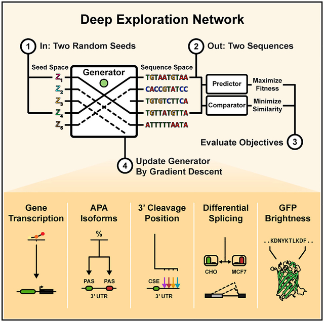
A generative neural network jointly optimizes fitness and diversity in order to design maximally strong polyadenylation signals, differentially used splice sites among organisms, functional GFP variants, and transcriptionally active gene enhancer regions.

INTRODUCTION

Designing DNA sequences for a target cellular function is a difficult task, as the cis-regulatory information encoded in any stretch of DNA can be very complex and affect numerous mechanisms, including transcriptional and translational efficiency, chromatin accessibility, splicing, 3′ end processing, and more. Similarly, protein design is challenging due to the non-linear, long-ranging dependencies of interacting residues. Yet, sequence-level design of genetic components and proteins has been making rapid progress in the past few years. Part of this advancement can be attributed to the collection of large biological datasets and improved bioinformatics modeling. In particular, deep learning has emerged as state of the art in predictive modeling for many sequence-function problems (Alipanahi et al., 2015; Zhou and Troyanskaya, 2015; Quang and Xie, 2019; Avsec et al., 2019; Kelley et al., 2016, 2018; Greenside et al., 2018; Jaganathan et al., 2019; Cuperus et al., 2017; Eraslan et al., 2019). These models are now beginning to be combined with design methods and high-throughput assays to forward-engineer DNA and protein sequences (Rocklin et al., 2017; Biswas et al., 2018; Sample et al., 2019; Bogard et al., 2019). The ability to code regulatory DNA and protein function could prove useful for a wide range of applications. For example, controlling cell-type-specific transcriptional, translational, and isoform activity would enable engineering of highly specific delivery vectors and gene circuits. Functional protein design, e.g., generating heterodimer binders or proteins with optimally stable 3D structures, could prove transformative in T cell therapy and drug development.

Discrete search heuristics such as genetic algorithms have long been considered the standard method for sequence design (Eiben and Smith, 2015; Shukla et al., 2015; Mirjalili et al., 2020). Recently, however, deep generative models, such as variational autoencoders (VAEs) (Kingma and Welling, 2013), autoregressive models, and generative adversarial networks (GANs) (Goodfellow et al., 2014), have been adapted for biomolecules (Riesselman et al., 2019; Costello and Martin, 2019; Repecka et al., 2019). Methods based on directed evolution have been proposed to condition such generative models for a target biological property (Gupta and Zou, 2019; Brookes et al., 2019).

Alternatively, differentiable methods based on activation-maximization can directly optimize sequences for maximal fitness by gradient ascent through a neural network fitness predictor. At its core, sequence design via gradient ascent treats the input pattern as a position weight matrix (PWM). A neural network, pre-trained to predict a biological function, is used to evaluate the PWM fitness. The gradient of the fitness score with respect to the PWM parameters is used to iteratively optimize the PWM by gradient ascent. This class of algorithms, applied to sequences, was first employed to visualize transcription factor-binding motifs learned from chromatin immunoprecipitation sequencing (ChIP-seq) data (Lanchantin et al., 2016). A modified version of the algorithm, with gradient estimators to allow passing sampled one-hot coded patterns as input, was used to design alternative polyadenylation (APA) sites (Bogard et al., 2019). The method has also been used to indirectly optimize sequences with respect to a fitness predictor by traversing a pre-trained generative model and iteratively updating its latent input (Killoran et al., 2017).

Gradient ascent-style sequence optimization is a continuous relaxation of discrete nucleotide-swapping searches and as such makes efficient use of neural network differentiability; rather than naively trying out random changes, we follow a gradient to make stepwise local improvements on the fitness objective. Still, the basic method has a number of limitations. First, it might get stuck in local minima and the fitness of the converged patterns is dependent on PWM initialization (Bogard et al., 2019). Second, it is computationally expensive to re-run gradient ascent for every sequence to generate. Third, the method has no means of controlling the diversity of optimized sequences. However, generating large, diverse sets of sequences might be necessary, given that the predictor has been trained on finite empirical data and will likely incorrectly score certain sequences. Methods that generate diverse sequences effectively increase the likelihood that some candidates have high fitness when tested experimentally.

To address these limitations, we developed deep exploration networks (DENs), an activation-maximizing generative neural network capable of optimizing sequences for a differentiable fitness predictor. The core contribution of DENs is to explicitly control sequence diversity during training. By penalizing any two generated sequences on the basis of similarity, we force the generator to traverse local minima and explore a much larger region of the cost landscape, effectively maximizing both sequence fitness and diversity (Figure 1A). Because DENs are parametric models, we can efficiently sample many sequences after having trained the generator. The architecture shares similarities with Killoran et al. (2017) but instead of optimizing the latent input seed of a pre-trained GAN, we optimize the weights of the generator itself for any pair of input seeds.

Figure 1. DEN Architecture.

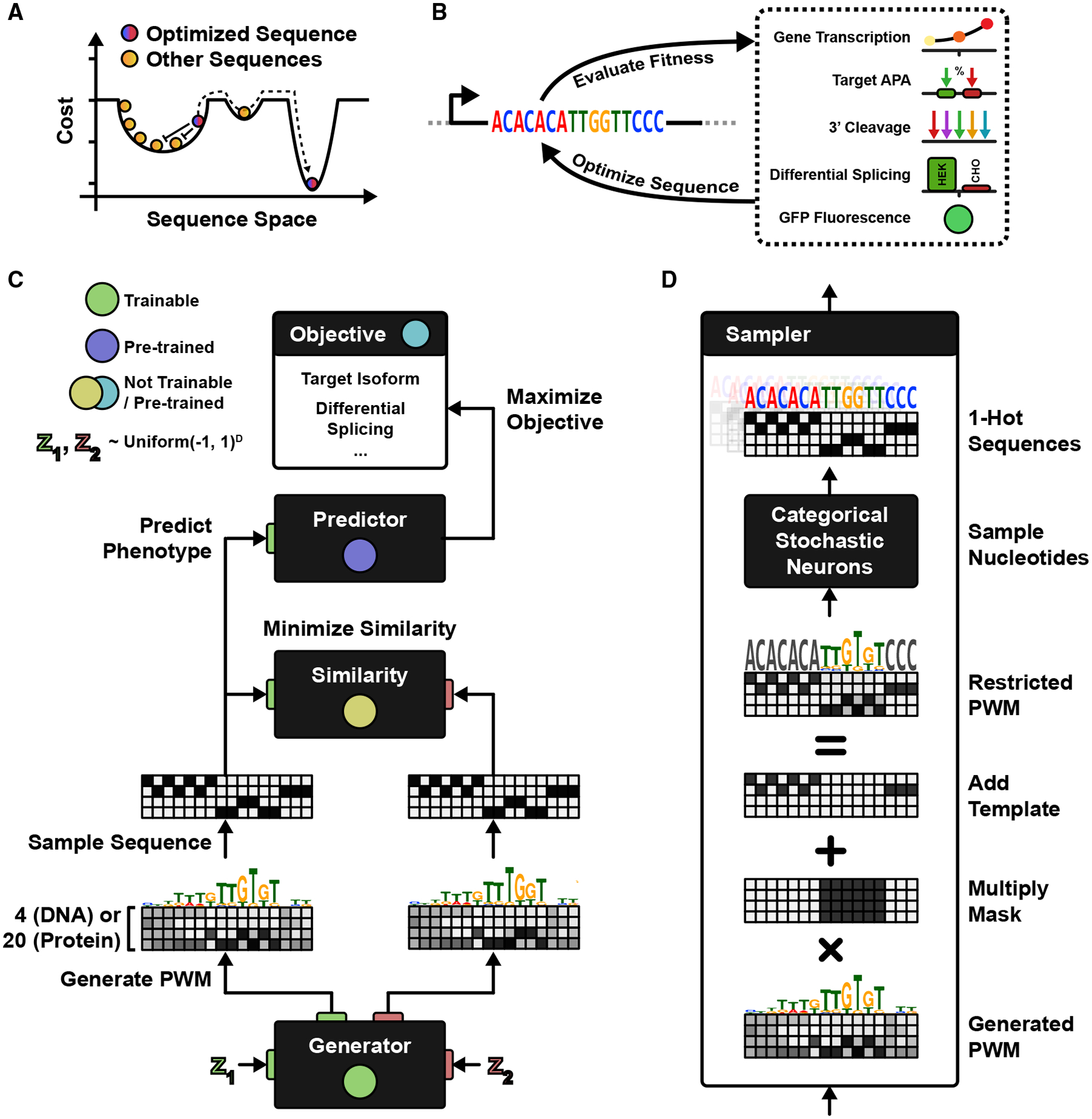
(A) A sequence produced by an input seed to a generative model (red-blue) shares the cost landscape with other generated sequences (orange). Patterns are penalized by similarity during training, resulting in an updated generator that transforms the red-blue seed into a different sequence, away from other patterns and potentially toward a new local minimum.

(B) Sequences are optimized on the basis of a pre-trained fitness predictor for some target function. We consider five different engineering applications: maximizing gene transcription, maximizing APA isoform selection, targeting 3′ cleavage positions, designing differential splicing between organisms, and improving green fluorescent proteins.

(C) In DENs, the generator is executed twice (independently) on two random seeds (z₁, z₂), producing two sequence patterns. One of the patterns is evaluated by the predictor, resulting in a fitness cost. The two patterns are also penalized on the basis of a similarity cost, and the generator is updated to minimize both costs.

(D) The PWM is multiplied by a mask (zeroing fixed nucleotides), and a template is added (encoding fixed letters). One-hot-coded patterns are outputted by sampling nucleotides from stochastic neurons, and gradients are propagated by straight-through estimation.

See also Figure S1.

For specific design tasks, the fitness predictor might quickly lose its predictive accuracy when the generated sequences move away from the training data in sequence space, making unbounded optimization of the predictor ill-suited. For example, stably folding proteins reside along a narrowly defined manifold in the space of all possible sequences and most protein datasets only contain measurements on this manifold. To overcome this issue, we integrate importance sampling of VAEs into the differentiable training pipeline of DENs, which allows us to maintain the likelihood ratio, or confidence, in generated sequences with respect to the measured data.

We evaluate the utility of DENs on several synthetic biology applications (Figure 1B): first, we develop a basic model to generate 3′ UTR sequences with target APA isoform abundance. Second, we extend the model to do conditional multi-class generation in the context of guiding 3′ cleavage position. Third, we apply DENs to construct splice regulatory sequences that are predicted to result in maximal differential splicing between two organisms. Fourth, on the level of DNA regulation, we benchmark DENs against competing methods when designing maximally transcriptionally active gene enhancer sequences. Finally, we use DENs for rational protein design and demonstrate state-of-the-art results on the task of designing green fluorescent protein (GFP) sequences.

RESULTS

Exploration in Deep Generative Models

The DEN architecture is based around a generative neural network $\mathcal{G}$ and a differentiable fitness predictor $\mathcal{P}$ (Figure 1C). Given an input pattern x, $\mathcal{P}$ is used to predict a property $\mathcal{P}(x)$ that we wish to design new patterns for. Here, x is a DNA or protein sequence represented as a one-hot-coded matrix x ∈ {0, 1}^N×M, where N denotes sequence length and M the number of nucleotides (4) or amino acids (20). Given a D-dimensional seed vector $z\in {ℝ}^D$ as input, the generator $\mathcal{G}$ outputs an approximate one-hot-coded pattern $x(z)=f(\mathcal{G}(z))*M+T$, where f transforms the real-valued nucleotide scores generated by $\mathcal{G}$ into an approximate one-hot-coded representation, mask matrix M zeroes out fixed sequence positions, and template matrix T encodes fixed nucleotides (Figure 1D). The predictor output $\mathcal{P}(x(z))$ is used to define a fitness cost ${\mathcal{C}}_{\text{Fitness}}[\mathcal{P}(x(z))]$, and the overall goal is to optimize $\mathcal{G}$ such that the generated sequences minimize this cost. Only $\mathcal{G}$ is optimized, having pre-trained $\mathcal{P}$ to accurately predict the target biological function.

By strictly minimizing ${\mathcal{C}}_{\text{Fitness}}[\mathcal{P}(x(z))]$, the generator will likely only learn to produce one single pattern, regardless of z, given that it is trivially optimal to always output the pattern located at the bottom of the local fitness cost minimum. There might however exist much better minima. Additionally, as the predictor might be inaccurate for certain sequences, the generator should ideally learn to sample many diverse patterns with maximal fitness scores. The distinguishing feature of a DEN is to force the generator to map randomly sampled vectors from the D-dimensional uniform distribution U(−1, 1)^D to many different sequences with maximal fitness score. This is achieved by making the generator compete with itself; we run $\mathcal{G}$ twice at each step of the optimization for a pair of independently sampled seeds z⁽¹⁾, z⁽²⁾ ~ U(−1, 1)^D and penalize the generator on the basis of both the fitness cost ${\mathcal{C}}_{\text{Fitness}}\left[\mathcal{P}\left(x\left(z^{(1)}\right)\right)\right]$ and a diversity cost ${\mathcal{C}}_{\text{Diversity}}\left[x\left(z^{(1)}\right),x\left(z^{(2)}\right)\right]$ evaluated on the generated patterns x(z⁽¹⁾), x(z⁽²⁾):

$$\underset{\mathcal{G}}{\text{min}}\lambda \cdot {\mathcal{C}}_{\text{Fitness}}\left[\mathcal{P}\left(x\left(z^{(1)}\right)\right)\right]+(1-\lambda )\cdot {\mathcal{C}}_{\text{Diversty}}\left[x\left(z^{(1)}\right),x\left(z^{(2)}\right)\right]$$ (Equation 1)

This monte-carlo optimization differs from a classical GAN (Goodfellow et al., 2014), which is typically trained to minimize some cost $\mathcal{C}[\mathcal{D}(\mathbf{\text{Data}}),\mathcal{D}(\mathcal{G}(z))]$ such that an adversarial discriminator $\mathcal{D}$ cannot distinguish between the real data and the distribution generated by $\mathcal{G}$. Also note that, in contrast to Killoran et al. (2017) where optimization is done on a single input seed of a pre-trained GAN, ${\text{min}}_z{\mathcal{C}}_{\text{Fitness}}[\mathcal{P}(\mathcal{G}(z))]$, we optimize the generator itself for all pairs of generator seeds. As training progresses, the generator will become injective over different seeds z ~ U(−1, 1)^D. Consequently, we can sample diverse high-fitness sequences by drawing samples from U(−1, 1)^D and transforming them through $\mathcal{G}$.

We investigate several cost functions for ${\mathcal{C}}_{\text{Diversity}}[x\left(z^{(1)}\right),x\left(z^{(2)}\right)]$. First, a cosine distance is used to directly penalize one-hot patterns on the basis of the fraction of identical nucleotides, considering multiple ungapped alignments (Figures S1A and S1B). We found that allowing a fraction of the sequences to be identical up to an allowable margin without incurring any cost gives the best results. We also evaluate a latent diversity penalty, where sequences are implicitly penalized on the basis of similarity in a (differentiable) latent space. Here, we use one of the fully connected layers of the predictor $\mathcal{P}$ as a latent feature space, coupled with a cosine similarity cost function (Figures S1C and S1D).

The generator can be trained to minimize the compound cost of Equation 1 by using any gradient-based optimizer. We built the DEN in Keras (Chollet, 2015) and optimized the generator with Adam (Kingma and Ba, 2014). For all design tasks, we set the diversity cost coefficient (1 − λ) to a sufficiently large value such that the cost approaches the allowable similarity margin early in the training. Function f used above to transform the real-valued nucleotide scores generated by $\mathcal{G}$ into an approximate one-hot-coded representation x(z) must maintain differentiability. We investigate two methods for achieving this: (1) representing x(z) as a softmax-relaxed PWM (Killoran et al., 2017; Stewart et al., 2018), and (2) representing x(z) by discrete one-hot-coded samples and approximating the gradient by using a softmax straight-through estimator (Bengio et al., 2013; Courbariaux et al., 2016; Chung et al., 2016; Bogard et al., 2019). See STAR Methods for further details on cost functions, differentiable sequence representations, and DEN training.

Engineering APA Isoforms

We first demonstrate DENs in the context of APA. APA is a post-transcriptional 3′ end processing event where competing polyadenylation (polyA) signals (PASs) in the same 3′ UTR give rise to multiple mRNA isoforms (Figure 2A) (Di Giammartino et al., 2011; Tian and Manley, 2017). A typical PAS consists of a core sequence element (CSE), often the hexamer AATAAA, as well as diverse upstream and downstream sequence elements (USE, DSE). Cleavage and polyadenylation occur approximately 17 nt downstream of the CSE within the DSE. In a competitive situation with multiple PASs in the same 3′UTR, the sequence of each PAS is the major determinant of isoform selection. We used APA REgression NeT (APARENT)—a neural network for predicting APA isoform abundance—as the predictor (Bogard et al., 2019) (Figure S2A). The generator followed a DC-GAN architecture (Radford et al., 2015) (Figure S2B).

Figure 2. Engineering APA Isoforms.

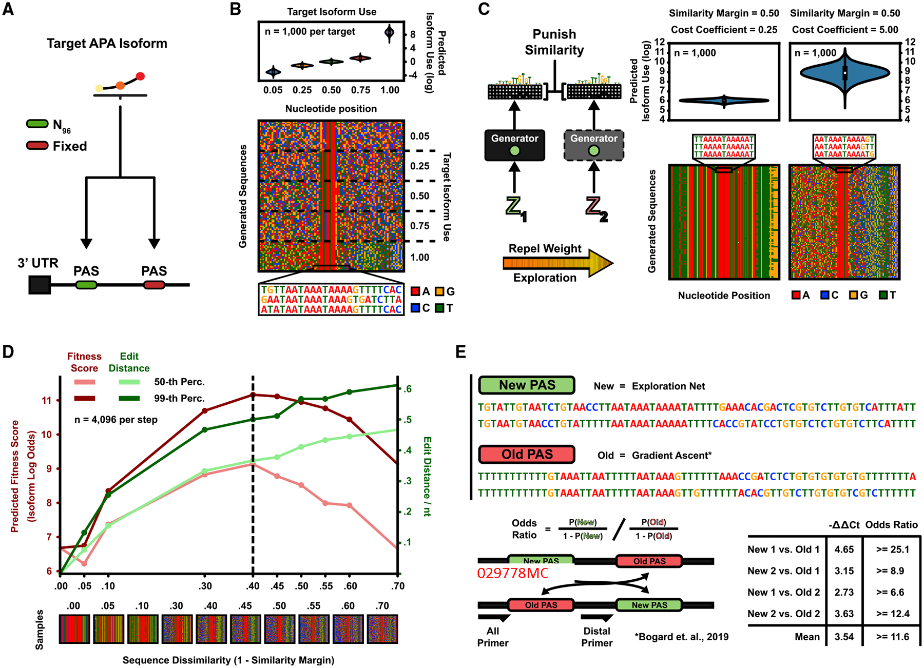
(A) Two PASs in a 3′ UTR compete for polyadenylation. The generative task is to design proximal PASs, which are selected at a target proportion.

(B) Five DENs were trained to generate sequences according to the APA isoform targets 5%, 25%, 50%, 75%, and 100% (“max”), with a sequence similarity margin (the fraction of nucleotides allowed to be identical) of 30% for the first four DENs and 50% for the max-target DEN. (Top) Predicted isoform proportions (n = 1,000 sequences per generator). Mean isoform proportion per generator (target in parenthesis): (5%) 5.25%, (25%) 25.06%, (50%) 50.6%, (75%) 74.2%, and (“max”) 99.98%. (Bottom) Pixel grid where rows denote sequences and columns nucleotide position (n = 20 sequences per generator). 0% duplication rate at 100,000 sampled sequences by any generator.

(C) The max-target DEN was re-trained with a low diversity cost coefficient (left) and a high coefficient (right). (Top) Predicted isoform proportions (n = 1,000 sequences). (Bottom) Sequence pixel grid (n = 100 sequences). Low coefficient (left): mean isoform log odds = 6.06, 99.5% duplication rate (n = 100,000 sequences). High coefficient (right): mean isoform log odds = 8.91, 0% duplication rate (n = 100,000 sequences).

(D) The max-target DEN was retrained for different values of the allowable sequence similarity margin. Plotted are the 50th/99th percentile of predicted fitness scores (isoform log odds) and pairwise normalized edit distances (n = 4,096 sequences per generator).

(E) Experiment validating the performance of the generated sequences. Two max-target sequences generated by the DEN were synthesized as either the proximal or distal PASon, a minigene reporter in competition with baseline gradient ascent-generated sequences (Bogard et al., 2019). Isoform odds ratios (preference fold changes) of the DEN PAS were assayed by using qPCR. Shown are the δδ cycle threshold values and associated odds ratios.

See also Figure S2; Videos S1 and S2.

We trained 5 DENs, each tasked with generating PASs according to the following target-isoform proportions: 5%, 25%, 50%, 75%, and maximal use (“max”); there was a 30% allowable similarity margin for the first four DENs and a 50% margin for the max-target DEN. In order to fit each generator to its target, we defined the fitness cost as the symmetric Kullback–Leibler (KL) divergence between the predicted and target-isoform proportion (Figure S2C; see STAR Methods for details). After training, each DEN could accurately generate sequences according to its objective (Figure 2B, top), as the mean of each generated isoform distribution was within 1% from the target proportion. The generated sequences for the max-target objective were predicted to be extremely efficient PASs (on average 99.98% predicted use). All five DENs exhibited a high degree of diversity (Figures 2B, bottom, S2D, and S2E; Videos S1 and S2); when sampling 100,000 sequences per generator, no two sequences were ever identical (0% duplication rate). Estimated from 1,000 sampled sequences, each generator had a hexamer entropy between 9.11 and 10.0 bits (of 12 bits maximum).

The optimization trajectories show that, as training progresses, the DENs immediately enforce sequence diversity (35%–45% normalized edit distance) whereas the fitness scores quickly converge to their optima within only 5,000 updates (Figure S2H). The trajectories also highlight differences when using one-hot samples with straight-through gradients, the continuous softmax relaxation, or a combination of both as input to the predictor. In general, the straight-through method consistently outperformed the softmax relaxation. The overall best configuration was achieved by using both representations and walking down the average gradient, with an explicit PWM entropy penalty. Using a nearest neighbor (NN) search, we also directly compared the DEN-generated sequences with PASs with measured isoform proportions from one of the massively parallel reporter assay (MPRA) training datasets (Bogard et al., 2019) (Figures S2F and S2G). The NN-inferred mean isoform proportion of each generator was close to its respective target (6.00%, 25.1%, 53.2%, and 73.7% respectively for targets 5%, 25%, 50%, and 75%), with a low standard deviation (between 3.03% and 7.18%). For the max-isoform target, the NN-inferred mean proportion was above the 99th percentile of measured values.

To evaluate the importance of exploration during training, we re-trained the max-isoform DEN with two different parameter settings; in one instance, we lowered the diversity cost coefficient to a small value, and in another instance, we increased it (Figure 2C). With a low coefficient, the generator only learned to sample few, low-diversity sequences, all of similar isoform log odds (Figure 2C, left; mean isoform log odds = 6.06, 99.5% duplication rate at 100,000 samples). With an increased coefficient, generated sequences became much more diverse and the mean isoform odds increased almost 20-fold (Figure 2C, right; mean isoform log odds = 8.91, 0% duplication rate). These results indicate that exploration during training drastically improves the final fitness of the generator. To find the optimal similarity penalty (for this design problem), we re-trained the max-isoform DEN under different similarity margins (the fraction by which we allow sequences to be similar), measuring the 50th and 99th percentile of fitness scores and sequence edit distances of each converged generator (Figure 2D). Both fitness and diversity increased up to a sequence dissimilarity of 40%. Beyond that point, the generated fitness scores monotonically decreased.

Finally, we evaluated the utility of promoting diversity in latent feature spaces. To this end, we re-trained the max-isoform DEN with an additional cosine similarity penalty enforced on the latent feature space of the fully connected hidden layer of APARENT (Figure S2I). Although the median fitness score dropped, the 99th percentile of generated scores remained above the 75th percentile of the original generator. Furthermore, the median normalized sequence edit distance increased from 38% to 50%. Interestingly, diversity in the latent space of an independently trained APA VAE also increased.

Experimental Validation of Deep Exploration Sequences

As suggested in Figures 2C and 2D, exploration increases the capability of generating high-fitness sequences. Next, we characterized DEN-generated PASs experimentally and compared their fitness with sequences generated by the baseline gradient ascent method. To that end, we synthesized APA reporters with two adjacent PASs (Figure 2E): each reporter contained one of the newly generated max-target PASs as well as one of the strongest gradient ascent-optimized signals from (Bogard et al., 2019). It is believed that the proximal PAS is slightly preferred compared with the distal PAS (Bentley, 2014). In order to discount this bias, we experimentally assayed both signal orientations where the DEN-generated PAS was either the proximal signal or the distal signal. The reporters were cloned onto plasmids and delivered to HEK293 cells. We quantified the expressed RNA isoform levels by using a qPCR assay, measuring the Ct values of total and distal RNA, respectively. Using Ct differences to estimate odds ratio lower bounds, we found that the DEN-generated sequences were on average 11.6-fold more preferred (usage odds increase) than the gradient ascent-generated sequences (Figure 2E). To put this in perspective, the strongest gradient ascent sequence had usage odds of 127:1 (99.22%) in relation to a distal bGH PAS separated by 200 nt. The DEN sequences would have usage odds of 1,481:1 (99.93%) in relation to the same signal.

A Comparison of Generative Models for Sequence Design

We carried out extensive benchmark comparisons between DENs and competing methods on three tasks (Figure 3A): (1) designing PASs for maximal polyadenylation isoform abundance (APARENT) (Bogard et al., 2019), (2) designing gene enhancer sequences for maximal transcriptional activity (MPRA-DragoNN) (Movva et al., 2019; Ernst et al., 2016), and (3) designing longer (1,000 nt) gene enhancer regions with maximal SPI1-binding score (DragoNN). We compared DENs with 6 competing methods: (1) GANs trained on the subset of the predictor’s data with the highest measured fitness score (Wang et al., 2019b), (2) activation-maximization of GANs (AM-GAN) (Killoran et al., 2017), (3) feedback-GANs (FB-GANs) (Gupta and Zou, 2019), (4) optimizing a single softmax-relaxed PWM by gradient ascent and sampling sequences from it (the baseline method), (5) optimizing several PWMs by gradient ascent, and (6) simulated annealing with the Metropolis acceptance criterion (Kirkpatrick et al., 1983; Metropolis et al., 1953). For FB-GAN, we tried using both a fixed feedback threshold (as in the original publication) as well as an adaptive threshold that was adjusted at each iteration. Only the two most competitive methods, DENs and simulated annealing, were compared on the third design task. See STAR Methods for further details. Fitness scores were compared to the median score of the baseline method (PWM gradient ascent), where the median score of random sequences was treated as 0% (i.e., −100%) of the baseline value.

Figure 3. Comparison of Sequence Design Methods.

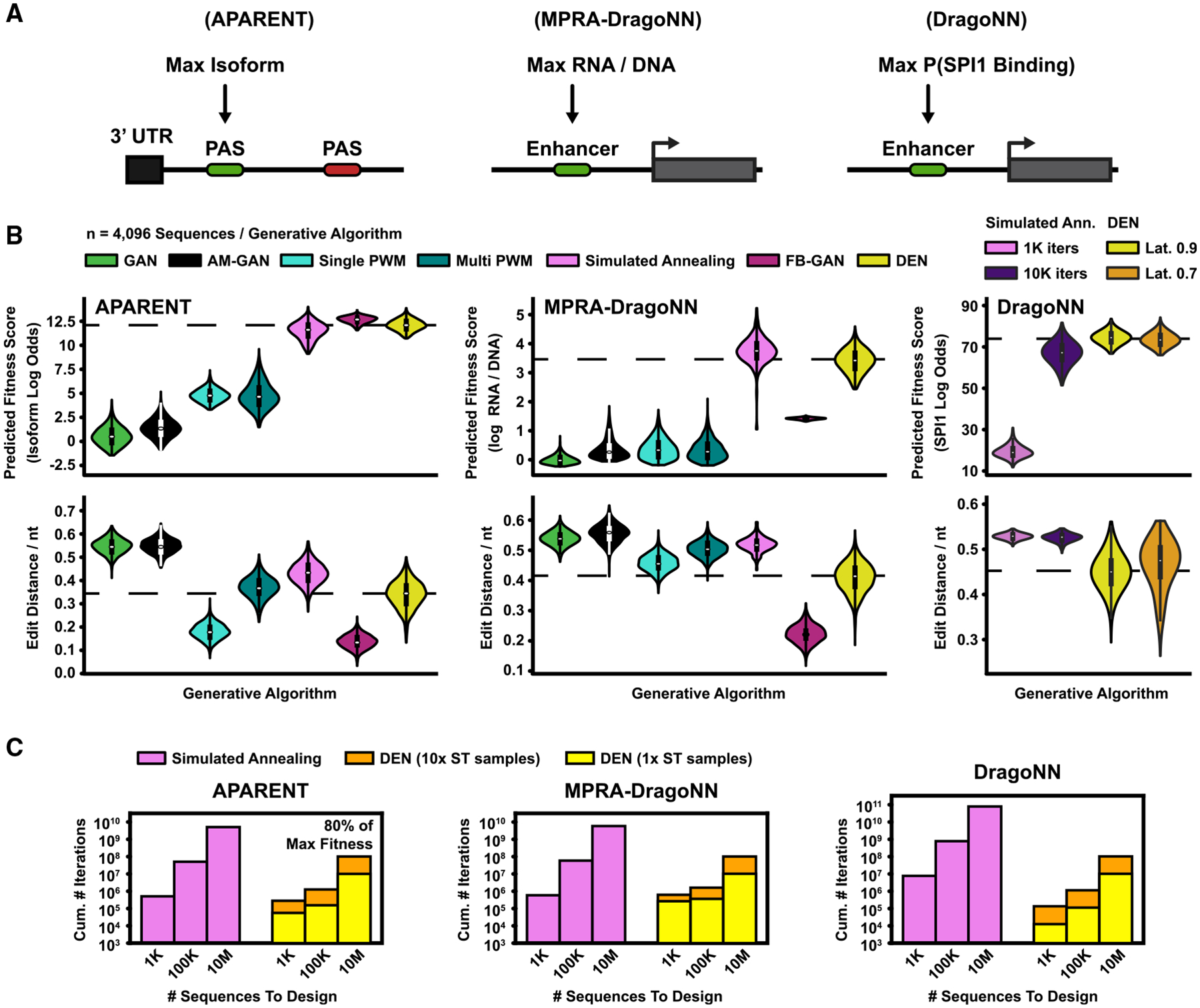
(A) Design methods were benchmarked on three tasks: (1) designing PASs with maximal isoform abundance (APARENT) (Bogard et al., 2019), (2) designing enhancer sequences for maximal transcription activity (MPRA-DragoNN) (Movva et al., 2019), and (3) designing sequences for maximal SPI1 binding (DragoNN).

(B) Seven design methods were evaluated (listed in top legend). Parametric models (GAN, FB-GAN, and DEN) were trained to convergence and subsequently used to sample n = 4,096 sequences. The GAN was trained on high-fitness data for each design task. FB-GAN and AM-GAN were based on GANs trained on a uniform subset of data. FB-GAN used an adaptive feedback threshold. DEN was trained with 50% sequence similarity margin for the first two design tasks (APARENT and MPRA-DragoNN). For the final task (DragoNN), we tried two latent penalties (70% or 90% margin). Per-sequence methods (AM-GAN, PWM Gradient Ascent, and simulated annealing) were re-initialized and optimized n = 4,096 times. (Top) Predicted fitness scores. (Bottom) Normalized pairwise sequence edit distances. Dashed lines indicate DEN median scores. See also Figures S3C–S3F.

(C) Extrapolated cumulative number of iterations (total sequence budget; y axis) required by DEN and simulated annealing to generate 1,000, 100,000, and 10,000,000 sequences (x axis) with a median predicted fitness score of 80% of the maximum value. Extrapolations were based on 960 optimized samples per method. We trained and evaluated two versions of DEN, where the number of one-hot samples used for the straight-through approximation during training was either 1 (yellow) or 10 (orange).

See also Figure S3.

For the APA design task, methods DEN, FB-GAN (with adaptive feedback threshold), and simulated annealing generated sequences with fitness score medians that were approximately +115% compared with baseline (Figures 3B, left, S3C, and S3D). However, sequence diversity was lower for FB-GAN (15% median normalized edit distance) compared with DEN (35%) and simulated annealing (45%). DEN-generated diversity could be increased by changing the allowable similarity margin, at the cost of diminished fitness scores (Figure S3C, left). However, the fitness scores were still higher than the majority of competing methods. Although sequence diversity increased for FB-GAN with fixed feedback threshold (45% median edit distance; Figure S3C, left), its median fitness score dropped significantly (−23% of the baseline median). Similarly, fitness scores were low for GAN and activation-maximization of GAN (−61.5% and −46.1% below baseline, respectively). Measured as the total number of sequences sampled during optimization, DEN converges to near-optimal fitness scores in fewer iterations than all other methods (Figure S3C, right). The results were more pronounced for the gene enhancer design task (Figures 3B, middle, S3E, and S3F): fitness score medians were +600% and +660% compared with baseline for DEN and simulated annealing respectively, whereas FB-GAN had a median score of +200%. DEN had approximately 3% lower median edit distance compared with baseline, but it was 17% higher compared with FB-GAN. Overall, DEN and simulated annealing generated sequences of comparable fitness, but simulated annealing was more diverse (between 7% and 10% increased edit distance). In fact, simulated annealing is a meta-heuristic known to find near-global minima given enough iterations (Wales and Doye, 1997), and the method optimally finds diverse basins by starting from random sequences. But simulated annealing is fundamentally more computationally expensive when generating many samples; the method must be re-initialized and optimized for every sequence to make. For the first two design tasks, extrapolations show that DEN can generate 100,000 sequences in fewer iterations (total sequence budget) than simulated annealing, which requires a similarly sized budget to produce only 1,000–10,000 sequences of comparable fitness (Figures 3C and S3G; the exact improvement depends on whether we use multiple one-hot samples for the straight-through approximation during DEN training). For the third task where sequences are longer, DEN can generate 10 million sequences with the same sequence budget simulated annealing requires for 1,000–10,000 sequences (Figures 3B, right, and S3G, right).

Engineering 3′ Cleavage Position

The next design task is closely related to APA, but rather than multiple competing PASs, we here concern ourselves with the position of 3′ cleavage within a single signal (Figure 4A). Cleavage occurs downstream of the central polyadenylation element—the CSE hexamer—however, the exact position and magnitude are tightly regulated by a complex code (Elkon et al., 2013). The predictor used for APA above—APARENT—can also predict the 3′ cleavage distribution, and so we re-use the model here (Figures S4A and S4B). Tasked with generating sequences that maximize cleavage at 9 distinct positions, we constructed a multi-class exploration network with a generator architecture similar to class-conditional GANs (Mirza and Osindero, 2014) (Figures 4B and S4C), where an embedding layer transforms the class label (target cut position) into a feature vector, which is concatenated onto every layer of the generator. We specify the fitness cost as the negative log likelihood of cleaving at the target position (given the predicted cleavage distribution of generated sequences).

Figure 4. Engineering 3′ Cleavage Positions.

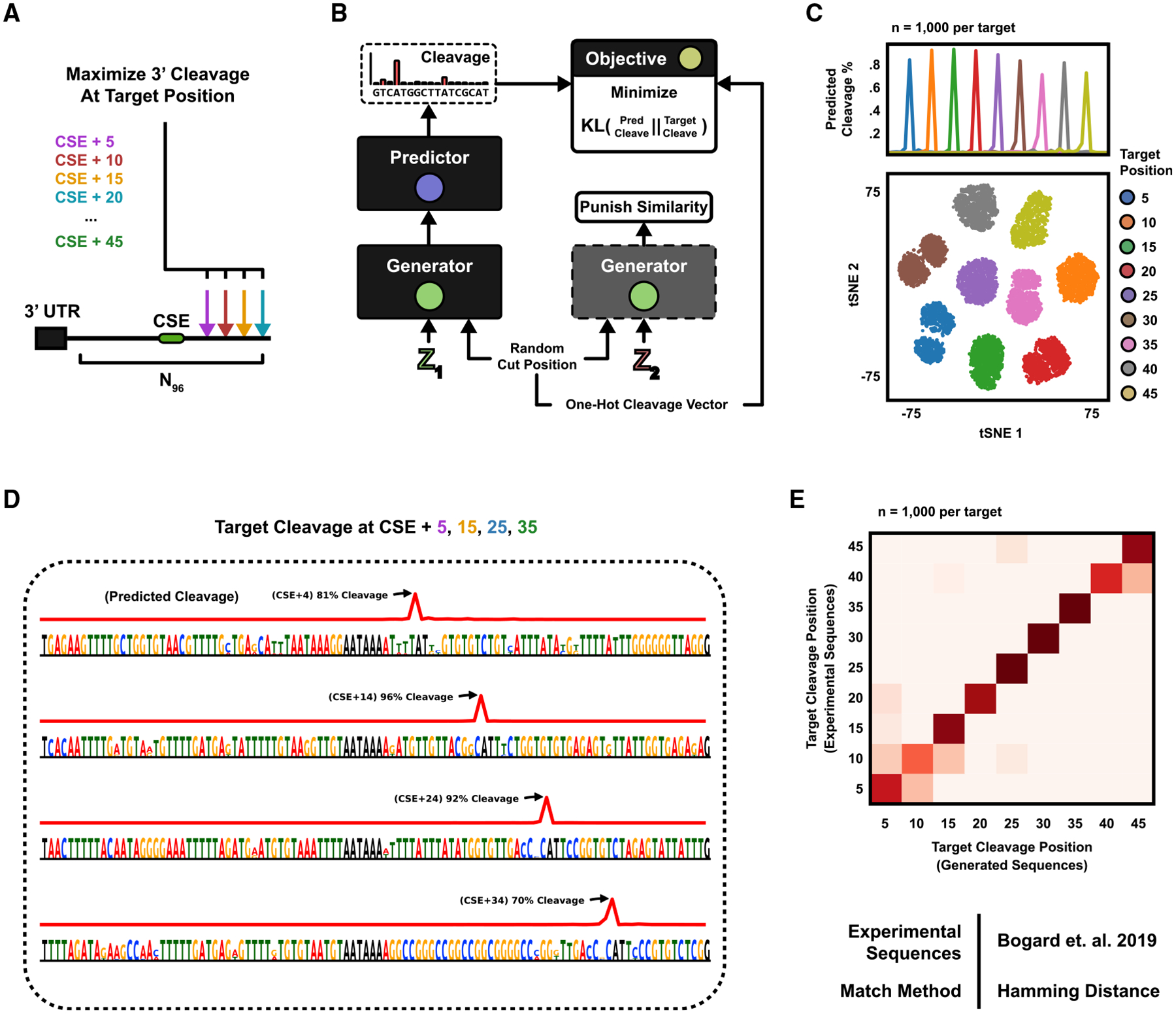
(A) The 3′ mRNA cleavage position is governed by a cis-regulatory code within the PAS. The generative task is formulated as designing PASs, which maximize cleavage at target nucleotide positions downstream of the central hexamer (CSE) AATAAA.

(B) A class-conditional DEN is optimized to generate sequences that are predicted to cleave according to a randomly sampled target cut position. The sampled cut position is also supplied as input to the generator.

(C) The DEN was trained to generate sequences with maximal cleavage at 9 positions, +5 to +45 nt downstream of the CSE, with 50% similarity margin. (Top) Mean predicted cleavage profile (n = 1,000 sequences per target position). Predicted versus target cut position R² = 0.998. (Bottom) All 9,000 sequences were clustered in tSNE and colored by target position.

(D) Example sequences generated for target positions +5, +15, +25, and +35. 0% duplication rate (n = 100,000 sequences). Hexamer entropy = 9.07 of 12 bits.

(E) The newly generated sequences were compared against gradient ascent-generated sequences for the same target (Bogard et al., 2019) by defining each cluster centroid as the mean one-hot pattern of all DEN-generated sequences and assigning each gradient ascent-pattern to the closest centroid on the basis of L1 distance. Agreement = 0.87.

See also Figure S4; Videos S3 and S4.

After training, the generator could sample diverse sequences with highly specific cleavage distributions given an input target position (Figures 4C and 4D; predicted versus target cut position R² = 0.998, 0% duplication rate at 100,000 sampled sequences; Figures S4D–S4F; Videos S3 and S4). When clustering the sequences in t-distributed stochastic neighbor embedding (tSNE) (Maaten and Hinton, 2008) (Figure 4C, bottom), we observe clearly separated clusters based on the target cleavage position. We further confirmed the function of the sequences by comparing them with a set of gradient ascent-optimized sequences, which had previously been validated experimentally with RNA-seq (Bogard et al., 2019) (Figure 4E; nearest neighbor agreement = 87%).

Engineering Proteins with Likelihood-Bounded Exploration Networks

The current DEN formulation maximizes fitness and diversity without regard to how confident the predictor (or any other model) is in the generated sequences. However, assuming the predictor loses its predictive power as the generated sequences drift from the measured training data in design space, it becomes necessary to maintain the marginal likelihood of sequences with respect to the data. This problem is particularly evident in protein design, where functional sequences are thought to reside in a manifold much smaller than the space of all possible sequences, and where measured training data only span this manifold. A related design method based on in silico directed evolution, conditioning by adaptive sampling (CbAS) (Brookes et al., 2019), controls the likelihood by adaptively sampling and retraining a VAE. Here, we integrate VAEs in the DEN framework (Figures 5A and S5A), enabling direct control of the approximate likelihood ratio of generated sequences with respect to a reference likelihood estimated on the training data. This allows us to tune, during backpropagation, how “confident” the DEN should be in the generated sequences (Figure 5B). We estimate the expected log likelihood of generated sequences by using importance sampling (Owen, 2013; Kingma and Welling, 2013; Blei et al., 2017) (see STAR Methods for details) and apply straight-through gradient estimation to optimize the generator for an additional likelihood ratio penalty with respect to the median training data likelihood. We validated this likelihood cost on the maximal APA design task (Figures S5B–S5D). By training two VAE instances on a subset of low- and high-fitness sequences, respectively, we confirmed that the likelihood cost restricted DEN optimization only when using the low-fitness VAE (which is expected when tasked with generating high-fitness samples).

Figure 5. Engineering Fluorescent Proteins with Likelihood-Bounded DENs.

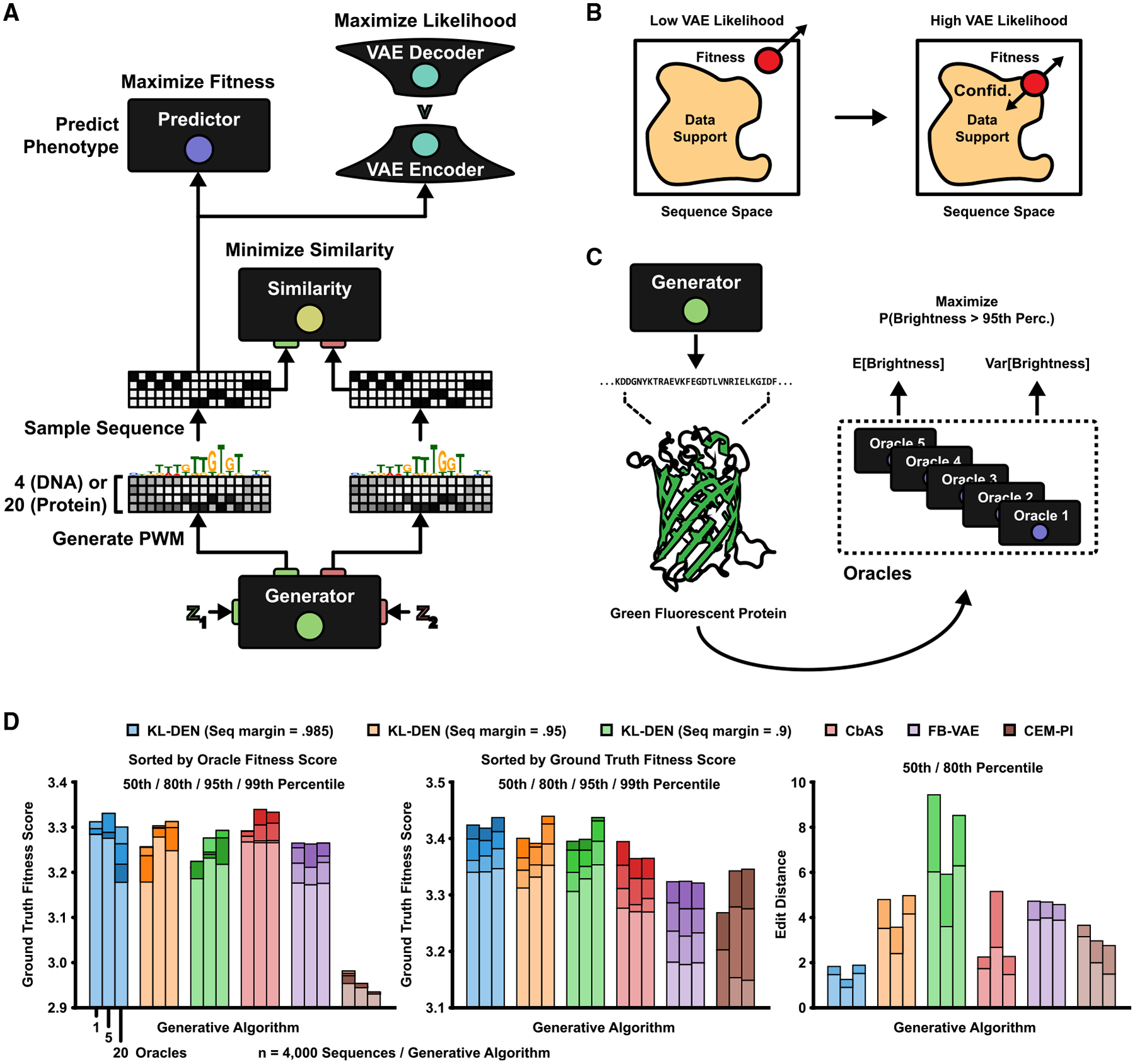
(A) The integration of a VAE in the DEN framework (KL-DEN). The one-hot-coded sequence patterns sampled from the generator are passed to the VAE. Gradients are backpropagated by using a straight-through estimator (Chung et al., 2016).

(B) Left: unbounded DEN optimization along the fitness gradient. Right: bounded optimization with a gradient pointing toward the VAE likelihood of the measured data.

(C) The task is to generate GFP sequence variants that maximize the predicted probability of their brightness being above a target (95th percentile of training data). Predictions are made by using an ensemble of oracles (Lakshminarayanan et al., 2017; Brookes et al., 2019).

(D) GFP benchmark comparison (methods listed in top legend). The KL-DEN was trained with a minimum likelihood ratio margin of 1/10 compared with the median training data likelihood, with three different sequence similarity margins: 98.5%, 95%, and 90%. Each method was used to sample 100 sequences per training epoch, for a total of 40 epochs (after 10 epochs of “warm up” training), resulting in n = 4,000 sequences. (Left) Sequences were sorted on oracle fitness scores. Shown are the “ground truth” scores for the 50th, 80th, 95th, and 99th percentile of oracle scores, as estimated by a GP regression model (Shen et al., 2014). (Middle) The 50th, 80th, 95th, and 99th percentile of ground truth scores (regardless of oracle value). (Right) 50th and 80th percentile of sequence edit distances.

See also Figure S5.

This KL-bounded DEN (abbreviated KL-DEN—given that its KL divergence with respect to the measured data are bounded) was benchmarked on the task of designing GFP sequences for maximal brightness, using variant data from Sarkisyan et al. (2016). Replicating the analysis of Brookes et al. (2019), we evaluated three increasingly large predictor ensembles (referred to as oracles) that enabled predicting the mean and variance of normalized brightness (Lakshminarayanan et al., 2017) (Figures 5C and S5E). We also changed the generator architecture by appending an long short term memory (LSTM) layer, as it increased convergence speed (Figure S5F). We tasked the KL-DEN with maximizing the probability of the predicted brightness being above the 95th percentile of the training data, while simultaneously enforcing generated sequences to be at least 1/10th as likely as the training data. We trained three KL-DEN versions with 98.5%, 95%, and 90% sequence similarity margins respectively. Performance was evaluated by using an independent Gaussian process regression model (Brookes et al., 2019; Shen et al., 2014) (considered the ground truth). We compared KL-DEN against CbAS, FB-VAE (a VAE-based version of FB-GAN) (Gupta and Zou, 2019), and CEM-PI (probability of improvement) (Snoek et al., 2012). The results showed that although KL-DEN was less consistent than CbAS (Figures 5D, left and S5G), it generated higher overall ground truth scores than those generated by CbAS, FB-VAE, and CEM-PI (Figures 5D, middle and S5H; 50th percentile of KL-DEN ground truth scores were consistently equal to or higher than the 80th percentile of CbAS scores). Furthermore, KL-DEN could generate more diverse sequences than all competing methods (Figures 5D, right, S5I; 80th percentile of edit distances were consistently higher for KL-DEN with 90% similarity margin). Finally, we compared against a regular DEN with no likelihood regularization penalty (Figure S5J). Although the predicted oracle scores increased rapidly, the DEN-generated ground truth values flatlined, highlighting the importance of maintaining the data likelihood to avoid overfitting to the oracle.

Engineering Organism-Specific Differential Splicing

Although precise cis-regulatory control in a single organism, cell type, or other condition has important applications, one of the hardest yet perhaps most interesting problems in genomics and synthetic biology is to code cis-regulatory functions that are differentially expressed across multiple cell types or conditions. Here, we consider the task of engineering organism-specific differential splice forms (Blencowe, 2006; Roca et al., 2013; Lee and Rio, 2015) (Figure 6A). Specifically, we define the task as maximizing the difference in splice donor usage (PSI) for an alternative 5′ splicing event in two different cell lines, by designing the regulatory sequences (25 nt) downstream of each alternative donor. This particular splicing construct has been studied in the context of HEK293 cells (Rosenberg et al., 2015), where MPRA data measuring hundreds of thousands of variants were collected. To study differential effects across multiple cell lines and organisms, we report additional MPRA measurements of this splicing library in HELA, MCF7, and CHO cells, which we used together with the original HEK data to train a cell-line-specific 5′ splice site usage prediction network (Figures 6B and S6A). The trained network could accurately predict splicing isoform proportions on a held-out test (Figure S6B; mean R² = 0.88 across cell lines). The predicted difference in splice site usage between cell lines had a strong correlation with measured differences (Figure S6C; predicted versus measured dPSI R² ranged between 0.35 and 0.47 depending on cell line pair). We focused on MCF7 and chinese hamster ovary (CHO), as the largest average differential trend was observed between these two cell lines.

Figure 6. Engineering Differential Splicing across Organisms.

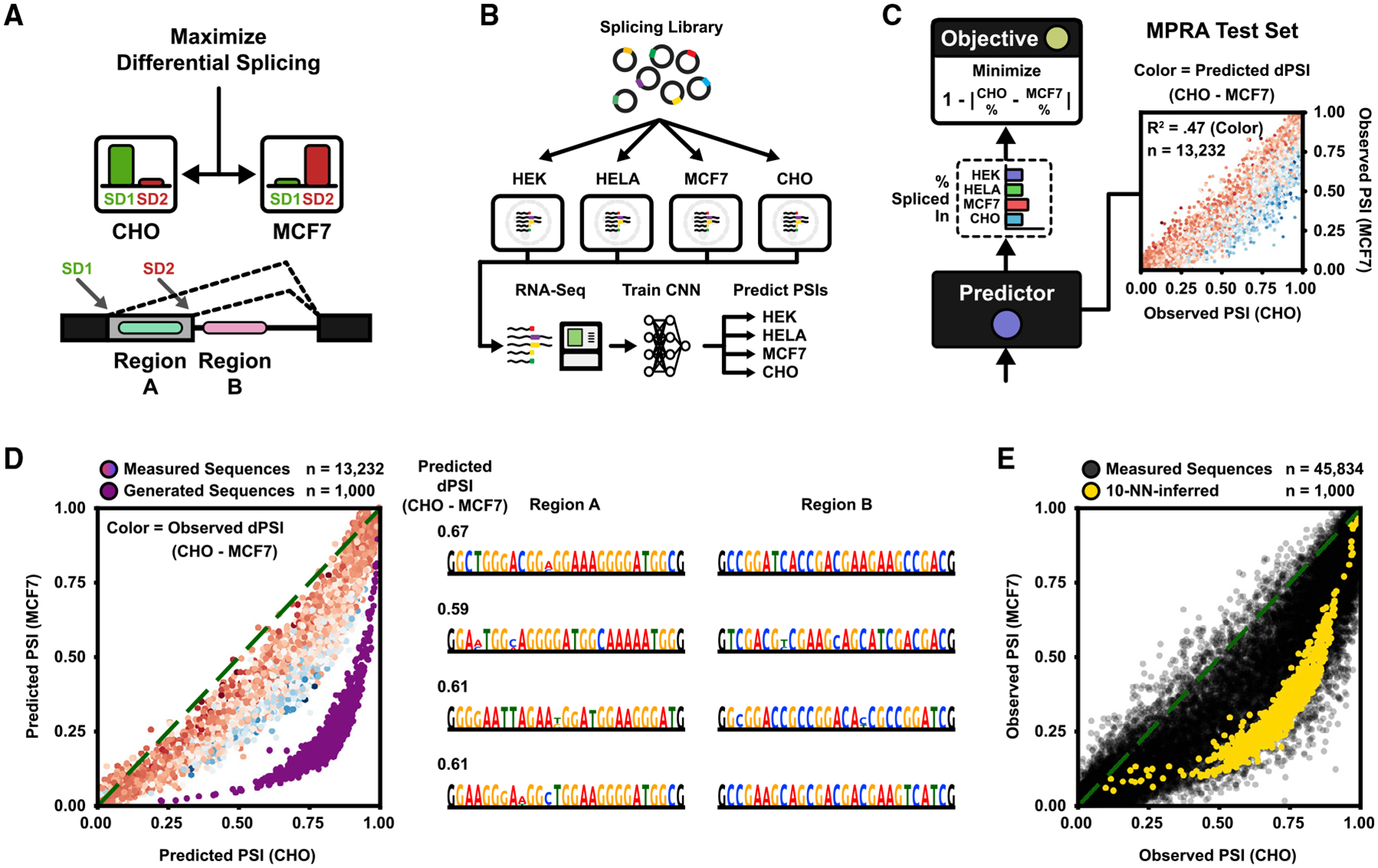
(A) Two 5′ splice donors compete for splicing. The task is to design two sequence regions, region A, which is located between the donors, and region B, which is located downstream of the 3′-most donor, to maximize differential usage (PSI) of donor 1 between two cell lines.

(B) Summary of the experimental pipeline. The MPRA of Rosenberg et al. (2015) was originally measured in HEK293 cells. Here, the library was replicated in additional cell lines HELA, MCF7, and CHO and measured by RNA-seq. A neural network (CNN) was trained on all four cell-line datasets to predict PSI per cell line given only the DNA sequence as input.

(C) (Left) The predicted MCF7 and CHO PSIs are used to maximize absolute difference. (Right) Measured MPRA test set PSIs for MCF7 and CHO. Color indicates predicted dPSI (blue or red = more or less used in CHO, respectively). Predicted versus measured delta PSI (dPSI) R² = 0.47.

(D) The DEN was trained to maximize dPSI between MCF7 and CHO, with 50% sequence similarity margin. (Left) Predicted PSI in MCF7 and CHO for generated sequences (purple; n = 1,000). Plotted are also the predicted PSI for MPRA test sequences (color indicates measured dPSI; n = 13,232). Mean predicted dPSI of test sequences = 0.08. Mean predicted dPSI of generated sequences = 0.56. (Right) Example generated sequences. 4% duplication rate (n = 100,000 sequences). Hexamer entropy = 8.31 of 12 bits.

(E) Validation of 1,000 generated sequences against the RNA-seq measured MPRA (n = 45,834) using nearest neighbors. The first dense layer of the fitness predictor was used as feature space (256 features). Measured PSIs of the entire MPRA (black) are plotted with the interpolated PSIs of the generated sequences (yellow), estimated from 10 neighbors. Mean MPRA dPSI = 0.07. Mean dPSI of generated sequences = 0.38.

See also Figure S6.

Next, we trained a DEN with the same generator architecture as in Figure 2B to maximize the difference in predicted organism-specific PSI (dPSI) between MCF7 and CHO (Figure 6C). We used the trained generator to sample 1,000 sequences, the majority of which were predicted to be far more differentially spliced than any of the sequences from the MPRA (Figure 6D; mean predicted dPSI of generated sequences = 0.56, compared with the average dPSI = 0.08 of the MPRA test set). For validation, we compared the generated sequences with the measured MPRA by using an NN search. We found that the DEN indeed learned to sample regulatory sequences centered on maximal differential splicing between the target cell lines (Figures 6E and S6D; mean NN-dPSI of generated sequences = 0.38, mean measured dPSI of MPRA sequences = 0.07).

Finally, we replicated the analysis by using a linear logistic regression model with hexamer counts as features rather than a convolutional neural network fitness predictor. By reducing the regression model to a set of differentiable tensor operations, we could seamlessly integrate the model in the DEN pipeline (Figures S6E and S6F). Allowing both high- and low-variance models enable more flexibility in tailoring the predictor properties for the given design task. In some applications it might even be suitable to compose predictor ensembles to increase rigidity. In our case, we could retrain the DEN to jointly maximize the neural network and hexamer regression predictors, striking a balance between the two models (Figure S6G).

DISCUSSION

We developed an end-to-end differentiable generative network architecture, DENs, capable of synthesizing large, diverse sets of sequences with high fitness. The model could generate PASs, which precisely conformed to target-isoform ratios and 3′ cleavage positions, differentially spliced sequences between two organisms (human MCF7 cells and hamster CHO cells respectively), maximally transcriptionally active gene enhancers, and even functional GFP variants. DENs control exploration during training by sampling two sequence patterns given two random seeds as input and penalizing sequence pairs that are similar above a certain threshold. Our analysis showed that the magnitude by which we punish similarity almost entirely determines final generator diversity and also largely determines the final fitness of the generated patterns. During training, the optimizer trades off exploring (repelling similar patterns) with exploiting (maximizing pattern fitness) on the basis of the temperature (diversity cost coefficient) until convergence is reached.

Benchmark comparisons showed that DENs produce more diverse, higher-fitness sequences than competing parametric generative models. Another concern in sequence design is computational efficiency; for some applications, we might want to generate millions of candidate patterns for high-throughput screening in the lab. As we demonstrated on several design tasks, DENs are fundamentally more efficient than per-sequence optimization methods, such as simulated annealing because, after paying the initial cost of training the DEN, we can sample new sequences with a single forward pass (scaling additively with the number of target sequences). For example, using a Tesla K80 GPU, it takes approximately 60 ms to predict a 64-sequence batch with the DragoNN model or 0.9 ms per sequence. Assuming that predictions make up most of the computational cost and that a single generator training pass takes 5 times longer than a batch prediction, then using the DEN from Figure 3C to generate 1 million sequences would take approximately 25,000 × 60 × 5 (training time) + 1,000,000 × 0.9 (design time) = 8,400,000 ms or 140 min. Using simulated annealing, which needed 10,000 iterations per sequence, would require roughly 1,000,000 × 10,000 × 0.9 = 9 billion ms or 100 days to finish.

DENs can be thought of as invertible networks for a highly surjective function value (namely maximal predicted fitness score). In fact, we can turn DENs into fully invertible regression models by making a few minor architectural changes. We demonstrate a proof of principle of an “inverse regression” DEN in Figure S7 (see STAR Methods for details). Current architectures of invertible neural networks are based around learning a bijective one-to-one mapping of the input data distribution to a latent code (Ardizzone et al., 2018). Inverse regression DENs similarly learn to map a simple latent space to the inverse domain (sequence) but without restrictions on the latent space or generator architecture. We also showed that DENs could be optimized to promote diversity not only by sequence-level comparison but also by latent similarity metrics. In particular, penalizing latent similarity in one of the fully connected predictor layers implicitly promoted diversity in the “true” latent feature space, as indicated by an independently trained VAE. In the case of differential splice sites, DENs could optimize sequences for both a neural network and hexamer regression predictor. The hexamer regression model, by its low-variance design, provides regularization. We further generalized the notion of regularization during DEN training, by incorporating a VAE. This allowed us to tune the likelihood ratio of generated sequences with respect to training data. We demonstrated competitive results against state-of-the-art cross entropy methods, such as CbAS (Brookes et al., 2019) and FB-GANs (Gupta and Zou, 2019). However, it is worth noting that the intended design cycle of CbAS differs fundamentally from DENs. CbAS is very sample efficient, which is important if we intend to experimentally measure generated sequences during training (the “oracle” is an actual experiment). By contrast, for DENs, we do not care much about the number of calls made to the oracle during training, as we assume it is always a differentiable predictor. Also note that, although simulated annealing was competitive with DENs when strictly maximizing a predictor, it is unclear if that method would even be applicable for this design task, as it is not obvious how a VAE would be incorporated.

In future work, there are several technical aspects to explore. First, the sequence diversity cost coefficient is currently kept constant. Although this efficiently enforces exploration, it might be too rigid in cases where cost landscapes have “pointy”—deep but narrow—valleys. By treating the diversity penalty as a temperature to anneal, or by changing the latent input distribution of the generator to allow a dynamic range of sequence similarity margins, DENs might be able to discover the pointy valleys during high-temperature periods of training and descend these during low-temperature periods. We also note that replacing the DC-GAN generator with a more complex model, for example, a deep residual network (He et al., 2016), might further increase the DEN’s capacity to learn diverse sequences.

Experimental assays provide us with powerful tools to validate sequences produced by generative models. Here, we tested a subset of our generated PASs. We observed that the new PASs were orders of magnitude stronger than any previously known sequence. In some applications, the initial predictor might not be sufficiently accurate, and the generated samples might reveal incorrect predictions once tested in the lab. Similar to earlier work on generative models employed for molecular design (Segler et al., 2018; Sample et al., 2019), DENs could be used with active learning, where the network generates a large set of candidate sequences, which, after synthesis and high-throughput measurements, provide augmented training data for the predictor, and this cycle is repeated until the generated patterns are in concordance with real biology. Beyond the design tasks covered here, there are many suitable biological applications for DEN. DENs could be used together with gene expression data to engineer cell-type-specific enhancer or promoter sequences with differential affinities. DENs might also prove useful for generating candidate CRISPR-Cas9 guide RNA with minimal off-target effects (Lin and Wong, 2018; Chuai et al., 2018; Wang et al., 2019a). Rational design of heterodimer protein pairs with orthogonal interaction has recently been demonstrated (Chen et al., 2019). As more data are collected and used to train functional models of interaction, we would be able to use DENs for generation of candidate orthogonal binder sets or even generalized interaction graphs. Finally, DENs could be coupled with models of protein structure (Senior et al., 2020; AlQuraishi, 2019) to generate stably folded proteins.

STAR★METHODS

RESOURCE AVAILABILITY

Lead Contact

Further information and requests for resources and reagents should be directed to and will be fulfilled by the Lead Contact, Johannes Linder (jlinder2@cs.washington.edu).

Materials Availability

This study did not generate new materials. The APA reporter plasmid backbone from (Bogard et al., 2019) was used for the polyadenylation qPCR assay. The plasmid backbone from (Rosenberg et al., 2015) was used for the splicing MPRA.

Data and Code Availability

The splicing MPRA dataset generated during this study is available at GitHub (https://github.com/johli/splirent). All original code is freely available for download at https://github.com/johli/genesis.

EXPERIMENTAL MODELS AND SUBJECT DETAILS

Four cell lines were used in this study: Human embryonic kidney cells (HEK293; female), human cervical cancer cells (HeLa; female), human breast cancer cells (MCF7; female), and chinese hamster ovary cells (CHO; female).

METHOD DETAILS

Experimental Methods

Here we describe the physical experiments reported in this study, including the polyadenylation qPCR reporter assay and the cell line-specific 5’ alternative splicing MPRA.

APA qPCR Reporter Assay

To evaluate the performance of the DEN-generated pA sequences, we experimentally compared two of the strongest newly generated sequences to two of the strongest gradient ascent-generated sequences from (Bogard et al., 2019).

Experiment

Each of the two DEN-generated pA sequences were constructed on plasmid reporters with one of the gradient ascent-sequences, such that they competed for polyadenylation when expressed in cells. Proximal pA signals have a preferential bias of selection compared to distal pA signals, so to discount this phenomenon we constructed two orientations of each reporter: In one orientation, the DEN-generated PAS was used as the proximal signal and the gradient ascent-generated PAS was the distal signal. In the other orientation, the gradient ascent-generated PAS was used as the proximal signal and the DEN-generated PAS was the distal signal. The plasmid reporters were identical to the APA reporters of (Bogard et al., 2019). See the Key Resources Table for plasmid maps.

KEY RESOURCES TABLE

REAGENT or RESOURCE	SOURCE	IDENTIFIER
Chemicals, Peptides and Recombinant Proteins
DMEM, high glucose, pyruvate	ThermoFisher Scientific	SKU#11995–065
Fetal Bovine Serum	Atlanta Biologicals	Cat#S11150
NEBNext Poly(A) mRNA Magnetic Isolation Module	New England Biolabs	Cat#E7490S
Fast Evagreen qPCR Master Mix	Biotium	Cat#31003
Opti-MEM Reduced Serum Medium	Invitrogen	Cat#22600050
Lipofectamine LTX Reagent with PLUS Reagent	Invitrogen	Cat#A12621
RNeasy	QIAGEN	Cat#74104
PolyA Spin mRNA Isolation Kit	New England Biolabs	Cat#S1560
MultiScribe Reverse Transcriptase	Invitrogen	Cat#4311235
Deposited Data
5’ Alternative Splicing MPRA	This study and Rosenberg et al., 2015	https://github.com/johli/splirent
APA Reporter Plasmids (qPCR Assay)	This study	https://github.com/johli/genesis/tree/master/analysis/apa/qpcr_experiment
Experimental Models: Cell Lines
HEK293FT	Invitrogen	Cat#R70007
HELA	ATCC	Cat#CCL-2.2
MCF7	ATCC	Cat#HTB-22
CHO-K1	ATCC	Cat#CCL-61
Software and Algorithms
DEN Software & Analysis	This study	https://github.com/johli/genesis
APA Predictor Software	Bogard et al., 2019	https://github.com/johli/aparent
Splicing Predictor Software	This study	https://github.com/johli/splirent
Feedback-GAN Software	Gupta and Zou, 2019	https://github.com/av1659/fbgan
CbAS Software & Benchmark	Brookes et al., 2019	https://github.com/dhbrookes/CbAS/
MPRA-DragoNN Software	Movva et al., 2019	https://github.com/kundajelab/MPRA-DragoNN
DragoNN (SPI1) Software	Kundaje Lab	https://github.com/kundajelab/dragonn

For each pair of competing signals, we measured the odds ratio of proximal isoform abundance of orientation 1 (DEN-signal is proximal) with respect to orientation 2 (gradient ascent-signal is proximal) using a qPCR assay, since this is equivalent to the fold change in selection preference for the DEN-generated signals. The plasmids were transfected in HEK293 cells and expressed for 48 hours before RNA extraction, following the protocol used in (Bogard et al., 2019). The total mRNA from each reporter were split into two samples – in one sample, we amplified both polyadenylation isoforms and in the other sample we selectively amplified only the distal isoform. For each sample, we used a universal forward primer (qPCR_FWD) and a variable reverse primer for PCR amplification. The reverse primer for each sample targeted either a sequence in the proximal PAS (qPCR_REV_upstream; amplifying both proximal and distal isoforms), or a sequence downstream of the proximal cleavage region (qPCR_REV_dnstream_A – qPCR_REV_dnstream_D; amplifying only the distally polyadenylated isoforms). See Table S1 for primer sequences. Cycle threshold (Ct) values of each qPCR experiment were read on a Biorad CFX.

Ct Difference Lower Bound On Isoform Odds Ratio

For each pair of reporters, we measure four different qPCR cycle threshold values:

1. ${\text{Ct}}_1^{all}$, the Ct for both proximal and distal RNA in reporter orientation 1.

2. ${\text{Ct}}_1^{\mathit{\text{distal}}}$, the Ct for both distal RNA only in reporter orientation 1.

3. ${\text{Ct}}_2^{all}$, the Ct for both proximal and distal RNA in reporter orientation 2.

4. ${\text{Ct}}_2^{\mathit{\text{distal}}}$, the Ct for both distal RNA only in reporter orientation 2.

Each cycle threshold value is inversely proportional to the log₂ of the RNA count, and so we can compute the following ΔCt values of log ratios:

$$\Delta {\text{Ct}}_1=-\left({\text{Ct}}_1^{\text{all}}-{\text{Ct}}_1^{\text{distal}}\right)={\text{log}}_2\left(\frac{p_1+d_1}{d_1}\right)$$

$$\Delta {\text{Ct}}_2=-\left({\text{Ct}}_2^{\text{all }}-{\text{Ct}}_2^{\text{distal }}\right)={\text{log}}_2\left(\frac{p_2+d_2}{d_2}\right)$$

Here, p₁ and d₁ are the proximal and distal RNA count of reporter orientation 1, p₂ and d₂ are the proximal and distal RNA count of reporter orientation 2, and ΔCt₁ and ΔCt₂ are the two reporters’ respective isoform log ratios. In the rest of this section, we prove that $2^{-\Delta \Delta \text{Ct}}=2^{-\left({\Delta \text{Ct}}_2-{\Delta \text{Ct}}_2\right)}$ is a lower bound on the isoform fold change, or Odds Ratio, of reporter 1 w.r.t. reporter 2. Using the definitions of ΔCt₁ and ΔCt₂ above, we have:

$$2^{-\Delta \Delta \text{Ct}}=2^{-\left(\Delta {\text{Ct}}_2-\Delta {\text{Ct}}_1\right)}=\frac{p_1+d_1}{d_1}/\frac{p_2+d_2}{d_2}$$

Next, define variables x₁ and x₂, the proximal isoform proportions of reporter 1 and 2:

$$x_1=\frac{p_1}{p_1+d_1}$$

$$x_2=\frac{p_2}{p_2+d_2}$$

We can rewrite our expression for 2^−ΔΔCt using only these variables:

$$\frac{p_1+d_1}{d_1}/\frac{p_2+d_2}{d_2}=\frac{1}{1-x_1}/\frac{1}{1-x_2}$$

Next, we multiply both of the smaller fractions with x₁ and x₂ on both sides, respectively:

$$\left(\frac{1}{x_1}\frac{x_1}{1-x_1}\right)/\left(\frac{1}{x_2}\frac{x_2}{1-x_2}\right)=\frac{x_2}{x_1}*\left(\frac{x_1}{1-x_1}/\frac{x_2}{1-x_2}\right)$$

We can now solve for the Odds Ratio in terms of 2^−ΔΔCt. At first glance, it appears we get a rest term x₁/x₂ that we cannot solve. However, we know from our experiments that and we previously derived that. In order for both these equations to be true, then, and as a consequence x₁/x₂>1. Hence, our measurements are proven to be lower bounds of the isoform odds ratio:

$$\text{Odds Ratio}\left(x_1,x_2\right)=\frac{x_1}{1-x_1}/\frac{x_2}{1-x_2}=\frac{x_1}{x_2}\cdot 2^{-\Delta \Delta \text{Ct}}>=2^{-\Delta \Delta \text{Ct}}$$

Cell Line-Specific Splicing MPRA

Previously unpublished repeat experiments of the alternative 5’ splicing MPRA from (Rosenberg et al., 2015) in additional cell lines HELA, MCF7 and CHO were used in this paper to study differential splicing trends and design maximally differentially used splice sites between CHO and MCF7. We outline the assay below and refer to the original publication for further details on the experimental protocol.

Experiment

The Citrine-based plasmid reporter library from (Rosenberg et al., 2015) was used, which contains two competing 5’ alternative splice donors with 25 degenerate bases inserted downstream of each splice donor. A degenerate barcode region is located in the Citrine 3’ UTR to enable mapping spliced mRNA back to originating plasmids. See the original publication for the plasmid map. Cell lines MCF7, HELA and CHO were cultured in DMEM on coated plates and transfected with the splicing library as described in (Rosenberg et al., 2015). RNA was extracted 24 hours after transfection and prepared for sequencing (Rosenberg et al., 2015). The purified mRNA library was sequenced on Illumina HiSeq2000, capturing both the 5’ splice junction of the degenerate intron and the barcode in the 3’ UTR. Finally, spliced and unspliced RNA reads were associated with the originating DNA plasmid based on the barcode from the sequenced 3’ UTR, enabling isoform count aggregation and Percent Spliced-In (PSI) estimation per unique library member.

After mapping and aggregating mRNA reads, the number of library members with non-zero read count in MCF7, CHO and HELA were 265, 016, 265, 010 and 264, 792 respectively. The mean read depth in these cell lines was 66.7, 72.0 and 29.1 respectively. (The previously described HEK293 dataset contained 265, 044 non-zero members with on average 50.0 reads per member).

Computational Methods

Here we present the computational methods developed and applied in this paper. We first describe the Deep Exploration Network (DEN) architecture, differentiable sequence representations, pattern masking operations and cost function definitions.

Next, we describe the sequence design tasks considered in this paper. For each task, we describe the predictor model used, the data it was trained on and the specific generator architecture used for training the DEN. Finally, for the benchmark comparison, we describe the details and parameter configuration of each design method tested.

Notation

The following notation is used:

• Scalars – Lowercase italic letters, e.g. c.

• Vectors and tensors – Lowercase bold italic letters, e.g. x.

• Scalar constants – Uppercase italic letters, e.g. N.

• Matrix and tensor constants – Uppercase bold letter, e.g. M.

• Subscripts are used to reference tensor elements, e.g x_ij.

• Parentheses are used to show implicit functional dependence, e.g. that x depends on z: x(z).

Definitions

The list below briefly summarizes the most important variables and entities defined in section ”Deep Exploration Network (DEN)” below. Note that there sometimes exist multiple independent instances of some of these variables, and we distinguish between variable instances using superscripts encased in parentheses (for example: x⁽¹⁾ and x⁽²⁾).

• $\mathcal{G}$ – Generator model function, i.e. $l=\mathcal{G}(z)$.

• z – Generator seed input.

• l – Generator output matrix (nucleotide log probabilities).

• $\mathcal{P}$ – Predictor model function, i.e. $y=\mathcal{P}(x)$.

• x – Sequence pattern (Either as PWM σ(l) or as one-hot sample δ(l)).

• σ(l) – PWM matrix obtained by softmax-normalizing l.

• δ(l) – one-hot-coded pattern sampled from σ(l).

Modeling and Optimization Software

We used the auto-differentiation and deep learning package Keras in Python for all neural network implementation and training (Chollet, 2015). For training the generator networks, we used the Adam optimizer (Kingma and Ba, 2014) with default parameters. To implement certain operations required during DEN training, we wrote custom code in Tensorflow (Abadi et al., 2016). The Tensorflow implementation for categorical straight-through gradient estimation (the one-hot sampling operation for sequence PWMs) was based on (Pitis, 2017).

Deep Exploration Network

Here we describe the model, cost function and training procedure of Deep Exploration Networks (DENs). For generator or predictor details, see the sections further below concerning specific applications.

Generator Architecture

The generator model $\mathcal{G}$ is a feed-forward neural network which receives a D-dimensional latent seed vector $z\in {ℝ}^D$ as input and outputs a real-valued pattern $l(z)=\mathcal{G}(z)\in {ℝ}^{N\times M}$. Here N denotes the number of letters of the generated sequence pattern and M denotes the number of channels (the alphabet size). In the context of genomics, the alphabet is the set of nucleotides and M = 4. The generated pattern l(z) is treated as a matrix of nucleotide logits. For some applications presented in this paper, the generator model takes auxiliary information as input in order to produce class-conditional patterns, in which case the formula can be described as $l(z)=\mathcal{G}(z,c)$, where c is either an integer representing the class index ($c\in \mathbb{N}$) or a real-valued scalar representing a target output value ($c\in ℝ$; for inverse regression).

An approximate one-hot-coded pattern x(z) is obtained by transforming the generated logit matrix l(z) through the formula:

$$x(z)=f(l(z))*M+T$$ (Equation 1)

Here f is a differentiable function which transforms the nucleotide logit matrix l(z) into an approximate one-hot-coded representation (function f detailed below). M and T are matrices used to mask and template the sequence pattern with fixed nucleotide content. This is useful if we want to bias the generation by locking particular motifs in the sequence. To support this, M masks the pattern by zeroing out fixed positions and T encodes the fixed sequence. M is constructed by encoding 1’s at changeable nucleotide positions and 0’s at fixed positions:

$$M_{ij}=\{\begin{array}{cc}1,& \text{if }i\text{ is not fixed}\\ 0,& \mathit{\text{else}}\end{array}$$ (Equation 2)

T is constructed by encoding 0’s at changeable nucleotide positions and a 1’s at every fixed position and column corresponding to the specific nucleotide identity:

$${\text{T}}_{ij}=\{\begin{array}{cc}1,& \text{if }i\text{ is fixed and }j\text{ encodes the nucleotide at position }i\\ 0,& \mathit{\text{else}}\end{array}$$ (Equation 3)

The exact architecture of the generator network depends on the application, but the overall design remains the same throughout the paper and is based on Deep Convolutional GANs (DC-GANs) (Radford et al., 2015) (see Figure S2B for a high-level illustration of the model). First, a dense layer with ReLU activations transforms the input seed $z\in {ℝ}^D$ into a high-dimensional vector. This vector is reshaped into a two-dimensional matrix, where the first dimension encodes sequence position and the second dimension encodes sequence channel. The position dimension is initially scaled down to a fraction of the final target sequence length, such that it can be upsampled by strided deconvolutions in subsequent layers. The channel dimension starts with a large number of channels and is gradually compressed to smaller numbers throughout the generator network, until the final layer outputs a sequence with only 4 channels (4 nucleotides). The de-convolutional layers are followed by convolutional layers. The filters vary in width between 6 and 8. All convolutional layers except the final layer have ReLU activations; the final layer has linear activations, corresponding to nucleotide log probabilities. We perform batch normalization between every convolutional layer.

Predictor Architecture

The goal of DENs is to generate diverse sequences which maximize some predicted biological fitness score. Given a one-hot coded sequence pattern x ∈ {0, 1}^N×M, $\mathcal{P}$ predicts a property $\mathcal{P}(x)$, which can be a real-valued score ($\mathcal{P}(x)\in ℝ$) or proportion ($\mathcal{P}(x)\in [0,1]$), and can be either scalar or multi-dimensional ($\mathcal{P}(x)\in {ℝ}^K$ for som K). The efficacy of x(z) is evaluated by a fitness cost function ${\mathcal{C}}_{\mathit{\text{Fitness}}}[\mathcal{P}(x)]$, based on the predicted property $\mathcal{P}(x)$ (further details below).

Any predictor $\mathcal{P}$ is compatible with Deep Exploration Networks as long as it is differentiable, i.e. the gradient ${\nabla }_x\mathcal{P}(x)$ must be defined (Simonyan et al., 2013; Lanchantin et al., 2016).

Training Procedure

In each forward pass, we sample two latent seed vectors z⁽¹⁾, z⁽²⁾ from the D-dimensional uniform distribution, z⁽¹⁾,z⁽²⁾ ~ U (−1, 1)^D. The seeds are independently passed as input to $\mathcal{G}$, generating two output patterns (nucleotide logit matrices) $l\left(z^{(1)}\right)=\mathcal{G}\left(z^{(1)}\right)$ and $l\left(z^{(2)}\right)=\mathcal{G}\left(z^{(2)}\right),$. Approximate one-hot-coded patterns x(z⁽¹⁾) and x(z⁽²⁾) are obtained by transforming l(z⁽¹⁾) and l(z⁽²⁾) through Equation 1. In its most basic form, the weights of the generator $\mathcal{G}$ are trained to minimize the following compound fitness and diversity cost function:

$$\underset{\mathcal{G}}{\text{min}}\lambda \cdot {\mathcal{C}}_{\text{Fitness}}\left[\mathcal{P}\left(x\left(z^{(1)}\right)\right)\right]+(1-\lambda )\cdot {\mathcal{C}}_{\text{Diversity}}\left[x\left(z^{(1)}\right),x\left(z^{(2)}\right)\right]$$ (Equation 4)

Here, ${\mathcal{C}}_{\text{Fitness}}\left[\mathcal{P}\left(x\left(z^{(1)}\right)\right)\right]$ is the fitness cost evaluated on the predicted property $\mathcal{P}\left(x\left(z^{(1)}\right)\right)$ and ${\mathcal{C}}_{\text{Diversity}}\left[x\left(z^{(1)}\right),x\left(z^{(2)}\right)\right]$ is the diversity cost evaluated on the patterns x(z⁽¹⁾),x(z⁽²⁾). In addition to these two cost components, DENs can optionally minimize two auxiliary losses: An entropy cost ${\mathcal{C}}_{\text{Entropy}}\left[\sigma \left(l\left(z^{(1)}\right)\right)\right]$ defined on a softmax relaxation σ(l(z⁽¹⁾)) and a regularization cost ${\mathcal{C}}_{\text{Reg}}\left[x\left(z^{(1)}\right)\right]$ (details below). We define the total DEN cost function ${\mathcal{C}}_{\text{Total}}\left[z^{(1)},z^{(2)}\right]$ as:

$${\mathcal{C}}_{\text{Total}}\left[z^{(1)},z^{(2)}\right]={\lambda }_F\cdot {\mathcal{C}}_{\text{Fitness}}\left[\mathcal{P}\left(x\left(z^{(1)}\right)\right)\right]+{\lambda }_D\cdot {\mathcal{C}}_{\text{Diversity}}\left[x\left(z^{(1)}\right),x\left(z^{(2)}\right)\right]+{\lambda }_E\cdot {\mathcal{C}}_{\text{Entropy}}\left[\sigma \left(l\left(z^{(1)}\right)\right)\right]+{\lambda }_R\cdot {\mathcal{C}}_{\text{Reg}}\left[x\left(z^{(1)}\right)\right]$$ (Equation 5)

λ_F, λ_D, λ_E, λ_R are the coefficients of each respective cost component.

The gradients ${\nabla }_{W_{\mathcal{G}}}l\left(z^{(1)}\right)={\nabla }_{W_{\mathcal{G}}}\mathcal{G}\left(z^{(1)}\right)$ and ${\nabla }_{W_{\mathcal{G}}}l\left(z^{(2)}\right)={\nabla }_{W_{\mathcal{G}}}\mathcal{G}\left(z^{(2)}\right)$ with respect to generator weights $W_{\mathcal{G}}$ can be computed with auto-differentiation in Keras, since the generator is a regular convolutional ReLU network. Also note that ${\nabla }_{l\left(z^{(1)}\right)}x\left(z^{(1)}\right)$ and ${\nabla }_{l\left(z^{(2)}\right)}x\left(z^{(2)}\right)$ are differentiable since we require the one-hot transform f from Equation 1 to be differentiable.

Differentiable Pattern Representation for Sequences

Equation 1 transforms the generated, real-valued, nucleotide logits $l=\mathcal{G}(z)\in {ℝ}^{N\times M}$ into an approximate one-hot-coded representation x(z) through function f. This representation must be carefully chosen in order to maintain differentiability with respect to $\mathcal{G}$. We investigate two different methods: (1) representing x(z) as a continuous, differentiable distribution, and (2) representing x(z) by discrete samples and approximating the gradient. The first pattern representation is referred to here as RIFR (Relaxed Input Form Representation), and is equivalent to a softmax-relaxed sequence PWM (Position Weight Matrix). We define the nucleotide-wise softmax function σ(l_ij) as:

$$\sigma \left(l_{ij}\right)=\frac{e^{l_{ij}}}{{\sum }_{k=1}^M{e}^{l_{ik}}}$$ (Equation 6)

Equation 6 transforms the generated logit matrices l(z⁽¹⁾) and lz⁽²⁾ into corresponding softmax-relaxed PWMs σ(l(z⁽¹⁾)) and σ(l(z⁽²⁾)) (Killoran et al., 2017). In RIFR, the PWMs σ(l(z⁽¹⁾)) and σ(l(z⁽²⁾)) are used as approximations for one-hot-coded patterns x(z⁽¹⁾) and x(z⁽²⁾) in the DEN cost function ${\mathcal{C}}_{\text{Total}}\left[z^{(1)},z^{(2)}\right]$. We redefine Equation 1 as:

$$x(z)=\sigma (l(z))*M+T$$ (Equation 7)

Note that in RIFR, the (masked) softmax-relaxed PWM σ(l(z⁽¹⁾)) is directly used as input to $\mathcal{P}$. Since Equation 7 is differentiable $\left(\frac{\partial \sigma \left(l_{ij}\right)}{\partial l_{ik}}=\sigma \left(l_{ik}\right)\cdot \left(1_{(j=k)}-\sigma \left(l_{ij}\right)\right)\right)$, an auto-differentiation package like Keras can compute the gradients ${\nabla }_{W_{\mathcal{G}}}x\left(z^{(1)}\right)$ and ${\nabla }_{W_{\mathcal{G}}}x\left(z^{(2)}\right)$. RIFR has a fundamental drawback: The predictor $\mathcal{P}$ has never been trained on real-valued patterns and may perform poorly on high-entropy PWMs. We can push the PWMs toward a one-hot-coded state during training by minimizing PWM entropy in the cost function. However, the gradient $\frac{\partial \sigma {(l)}_{ij}}{\partial l_{ik}}$ approaches zero as we explicitly minimize the entropy of the softmax probabilities. Put differently, we optimize the system for vanishing gradients, which may halt convergence.

The second pattern representation is referred to as SIFR (Sampled Input Form Representation) and consists of K discrete, one-hot-coded samples drawn from the PWMs σ(l(z⁽¹⁾)) and σ(l(z⁽²⁾)). Specifically, The nucleotide logits l(z)_ij are used as parameters to N independent categorical distributions ${ℂ}_i$, where the probability of sampling nucleotide j at position i is equal to the softmax value σ(l(z)_ij). Formally, we define the discrete one-hot sampling function δ as:

$$\begin{gathered} \delta \left(l_{ij}\right)=1_{\left(Z_i=j\right)} \\ \text{where }{Z}_i~{ℂ}_i=\text{Categorical}\left({\left\{p(k\mid l)=\sigma \left(l_{ik}\right)\right\}}_{k=1}^M\right) \end{gathered}$$ (Equation 8)

Using Equation 8, we sample K one-hot patterns x(z⁽¹⁾)^(k), x(z⁽²⁾)^(k) from l(z⁽¹⁾) and l(z⁽²⁾):

$$x{(z)}^{(k)}=\delta (l(z))*M+T$$ (Equation 9)

Finally, the cost function ${\mathcal{C}}_{\text{Total}}\left[z^{(1)},z^{(2)}\right]$ (Equation 5) is redefined as an empirical mean across all K sampled pairs $x{\left(z^{(1)}\right)}^{(k)}$ and $x{\left(z^{(2)}\right)}^{(k)}$:

$${\mathcal{C}}_{\text{Total }}\left[z^{(1)},z^{(2)}\right]=\frac{1}{K}\sum _{k=1}^K({\lambda }_F\cdot {\mathcal{C}}_{\text{Fitness}}\left[\mathcal{P}\left(x{\left(z^{(1)}\right)}^{(k)}\right)\right]+{\lambda }_D\cdot {\mathcal{C}}_{\text{Diversity}}\left[x{\left(z^{(1)}\right)}^{(k)},x{\left(z^{(2)}\right)}^{(k)}\right]+{\lambda }_E\cdot {\mathcal{C}}_{\text{Entropy}}\left[\sigma \left(l\left(z^{(1)}\right)\right)\right]+{\lambda }_R\cdot {\mathcal{C}}_{\text{Reg}}\left[x{\left(z^{(1)}\right)}^{(k)}\right])$$ (Equation 10)

The gradients ${\nabla }_{W_{\mathcal{G}}}x{\left(z^{(1)}\right)}^{(k)}$ and ${\nabla }_{W_{\mathcal{G}}}x{\left(z^{(2)}\right)}^{(k)}$ are approximated using the straight-through estimator of (Chung et al., 2016), where the gradient of δ is replaced by that of the softmax:

$$\frac{\partial \delta \left(l_{ij}\right)}{\partial l_{ik}}\approx \frac{\partial \sigma \left(l_{ij}\right)}{\partial l_{ik}}=\sigma \left(l_{ik}\right)\cdot \left(1_{(j=k)}-\sigma \left(l_{ij}\right)\right)$$ (Equation 11)

We implement custom operations in Keras/Tensorflow to compute Equation 11 during training (Bengio et al., 2013; Courbariaux et al., 2016; Pitis, 2017). The increased sample variance of SIFR can be mitigated by increasing the number of samples drawn (K). However, optimization can be noisy even with infinitely many samples (K → ∞), since straight-through gradients may at times be poor estimates of the gradient. As our results indicate in Figure S2H, combining both methods and walking down the average gradient (Dual Input Form Representation, or DIFR) can reduce variance and estimation artifacts.

Cost Functions

We minimize 4 costs when training a DEN:

1. A fitness cost ${\mathcal{C}}_{\text{Fitness}}\left[\mathcal{P}\left(x\left(z^{(1)}\right)\right)\right]$

2. A diversity cost ${\mathcal{C}}_{\text{Diversity}}\left[x\left(z^{(1)}\right),x\left(z^{(2)}\right)\right]$

3. An entropy cost ${\mathcal{C}}_{\text{Entropy}}\left[\sigma \left(l\left(z^{(1)}\right)\right)\right]$

4. A regularization cost ${\mathcal{C}}_{\text{Reg}}\left[x\left(z^{(1)}\right)\right]$.

Cost term: ${\mathcal{C}}_{\text{Fitness}}$

The predictor output $\mathcal{P}(x(z))$ is used to define a fitness cost ${\mathcal{C}}_{\text{Fitness}}[\mathcal{P}(x(z))]$. The choice of ${\mathcal{C}}_{\text{Fitness}}[\mathcal{P}(x(z))]$ is detailed in later sections for each specific design problem.

Cost term: ${\mathcal{C}}_{\text{Diversity}}$

The diversity cost ${\mathcal{C}}_{\text{Diversity}}\left[x\left(z^{(1)}\right),x\left(z^{(2)}\right)\right]$ can be any differentiable comparator function of the two generated patterns x(z⁽¹⁾) and x(z⁽²⁾). The standard diversity cost used throughout the paper is a sequence-level cosine similarity metric, which directly penalizes the patterns proportional to the fraction of identical nucleotides. To support translational invariance, we penalize patterns by the maximum cosine similarity across multiple offsets σ, ranging from σ = − σ_max to σ_max. The penalty is defined as a margin loss, allowing patterns to be identical up to a margin ϵ without incurring any cost. Given two masked one-hot coded patterns $x^{(1)}=f\left(\mathcal{G}\left(z^{(1)}\right)\right)*M$ and $x^{(2)}=f\left(\mathcal{G}\left(z^{(2)}\right)\right)*M$, we define the sequence similarity cost as:

$${\mathcal{C}}_S\left(x^{(1)},x^{(2)}\right)=\text{max}\left[-ϵ+\frac{1}{N^{*}}\underset{\sigma }{\text{max}}\sum _{i=1}^{N-\left|\sigma \right|}\sum _{j=1}^M{x}_{i+\text{max}(\sigma ,0),j}^{(1)}\cdot x_{i+\text{max}(-\sigma ,0),j}^{(2)},0\right]$$ (Equation 12)

Here, x⁽¹⁾ and x⁽²⁾ are masked by M (to zero out fixed positions) but not templated by T since fixed nucleotides should not affect the diversity penalty, and N* refers to the number of non-zeroed positions by M. N refers to the total sequence length and M the number of one-hot channels. Theoretically, we should set σ_max = N − 1 to test all possible offsets, however practically we found that σ_max = 1 was enough to remove offset artifacts.

When using RIFR (x⁽¹⁾ and x⁽²⁾ are softmax-relaxed PWMs), ${\mathcal{C}}_S\left(x^{(1)},x^{(2)}\right)$ is similar to an L2 penalty, where two sequence letters are penalized proportional to the magnitude of their PWM entries. When using SIFR (x⁽¹⁾ and x⁽²⁾ are one-hot samples), ${\mathcal{C}}_S\left(x^{(1)},x^{(2)}\right)$ corresponds to a sparse L1 penalty. For the tasks considered in this paper, we found that SIFR worked best. For all design tasks, we set the diversity cost coefficient to a sufficiently large value such that the cost reaches the allowable similarity margin ϵ early in the training. The margin ϵ is chosen by training the DEN for a range of values and selecting the setting with minimal fitness cost.

We also evaluate a latent diversity cost, which is defined on a pair of latent feature vectors u⁽¹⁾ and u⁽²⁾ obtained from the generated sequence patterns x⁽¹⁾ and x⁽²⁾ by applying some (differentiable) feature transform $u^{(1)}=\mathcal{M}\left(x^{(1)}\right)$ and $u^{(2)}=\mathcal{M}\left(x^{(2)}\right)$. In theory, $\mathcal{M}$ can be any type of encoder model, e.g. a variational autoencoder (VAE). In the paper, we let $\mathcal{M}$ be the subnetwork of predictor $\mathcal{P}$ ending at the first fully connected (dense) layer, i.e. we let the first fully connected layer of $\mathcal{P}$ be the latent feature space for u⁽¹⁾ and u⁽²⁾. We define the latent similarity cost as the cosine similarity margin loss between u⁽¹⁾ and u⁽²⁾:

$${\mathcal{C}}_{\text{L}}\left(u^{(1)},u^{(2)}\right)=\text{max}\left[\frac{{\sum }_{i=1}^d{u}_i^{(1)}\cdot u_i^{(2)}}{\sqrt{{\sum }_{i=1}^d{\left(u_i^{(1)}\right)}^2}\cdot \sqrt{{\sum }_{i=1}^d{\left(u_i^{(2)}\right)}^2}}-ϵ,0\right]$$ (Equation 13)

Cost term: ${\mathcal{C}}_{\text{Entropy}}$

We explicitly control the entropy of the generated softmax-relaxed PWM σ(l(z)) by fitting the Shannon Entropy to a target (or minimum) value. When fitting to a target conservation t_bits (bits), we minimize a squared error between the average nucleotide entropy and t_bits:

$${\mathcal{C}}_{\text{Entropy}}[\sigma (l(z))]={\left[t_{\text{bits}}-\frac{1}{N}\sum _{i=1}^N\left({\text{log}}_{2}M-\sum _{j=1}^M-\sigma \left(l{(z)}_{ij}\right)\cdot {\text{log}}_2\sigma \left(l{(z)}_{ij}\right)\right)\right]}^2$$ (Equation 14)

When enforcing a minimum average conservation m_bits, we minimize a margin cost instead:

$${\mathcal{C}}_{\text{Entropy}}[\sigma (\mathit{l}(\mathit{z}))]=\text{max}\left[m_{\text{bits}}-\frac{1}{N}\sum _{i=1}^N\left({\text{log}}_{2}M-\sum _{j=1}^M-\sigma \left(\mathit{l}{(\mathit{z})}_{ij}\right)\cdot {\text{log}}_2\sigma \left(\mathit{l}{\left(\mathit{z}\right)}_{ij}\right)\right),0\right]$$ (Equation 15)

Cost term: ${\mathcal{C}}_{\text{Reg}}$

We optionally penalize or reward specific motifs in the generated pattern by shifted multiplication with itself to mask out sub-patterns. This is useful for example to repress known artifacts of the predictor. Same as ${\mathcal{C}}_{\text{Diversity}}\left[x\left(z^{(1)}\right),x\left(z^{(2)}\right)\right]$, the regularization cost ${\mathcal{C}}_{\text{Reg}}[x(z)]$ can either be used with SIFR (sampled discrete one-hot patterns) to provide sparse regularization or with RIFR (softmax-relaxed PWMs), to support L2 penalties. We find that SIFR gives better results when penalizing motifs and RIFR gives better convergence for promoting motifs.

For each one-hot-coded motif F of length L, we either add or subtract ${\mathcal{C}}_{\text{motif}}[x(z),F]$ to/from ${\mathcal{C}}_{\text{Reg}}[x(z)]$, to penalize or promote generation of F respectively in positions [a, b] of x(z):

$${\mathcal{C}}_{\text{motif }}[x(z),F]=\sum _{i=a}^{b-L}x{(z)}_{i,\text{ argmax}\left({\text{F}}_1\right)}\cdot \dots \cdot x{(z)}_{i+L,\text{ argmax}\left({\text{F}}_L\right)}$$ (Equation 16)

Here argmax (F_j) corresponds to the nucleotide identity at the j:th position of F.

Variational Inference and KL-Bounded DENs

In the analysis presented in Figures 5 and S5, a variational autoencoder (VAE) was used to approximate and maintain the marginal likelihood p_Data(x(z)) of generated sequences x(z) with respect to the measured data. By specifying a minimum target likelihood ratio that must be upheld by the DEN during backpropagation, we avoid drift into low-confidence regions of sequence design space. Specifically, assuming we have trained a VAE such that p_VAE(x) ≈ p_Data(x), ∀x ∈ {0, 1}^N×M (see below for VAE training details), we estimate the expected log-likelihood ${\mathbb{E}}_z\left[\text{log }{p}_{VAE}(x(z))\right]$ of x(z) using importance sampling during the forward pass, and optimize $\mathcal{G}$ for all seeds z⁽¹⁾, z⁽²⁾ ~ U(−1, 1)^D by gradient descent to minimize:

$${\text{min}}_{\mathcal{G}}{\lambda }_F\cdot {\mathcal{C}}_{\text{Fitness}}\left[\mathcal{P}\left(x\left(z^{(1)}\right)\right)\right]+{\lambda }_D\cdot {\mathcal{C}}_{\text{Diversity}}\left[x\left(z^{(1)}\right),x\left(z^{(2)}\right)\right]+{\lambda }_E\cdot {\mathcal{C}}_{\text{Entropy}}\left[\sigma \left(l\left(z^{(1)}\right)\right)\right]+{\lambda }_L\cdot {\mathcal{C}}_{\text{Likelihood}}\left[{\mathbb{E}}_z\left[\text{log }{p}_{\text{VAE}}\left(x\left(z^{(1)}\right)\right)\right]\right]$$ (Equation 17)

Here ${\mathcal{C}}_{\text{Likelihood}}\left[{\mathbb{E}}_z\left[p_{\text{VAE}}(x(z))\right]\right]$ is a cost function defined in terms of the estimated expected log likelihood ${\mathbb{E}}_z[\text{log }{p}_{\text{VAE}}(x(z))]$ of x(z). The likelihood weight λ_L is to a sufficiently large value such that ${\mathcal{C}}_{\text{Likelihood}}\left[{\mathbb{E}}_z\left[p_{\text{VAE}}(x(z))\right]\right]$ quickly reaches 0 during training.

The expected log-likelihood ${\mathbb{E}}_z[\text{log }{p}_{\text{VAE}}(x(z))]$ is approximated in the forward pass during DEN training as follows: The (differentiable) one-hot sequence pattern x(z) generated by $\mathcal{G}$ (Equation 1) is used as input to the VAE encoder $\mathcal{E}$ producing a mean vector μ(z) ∈ R^D and a log-variance vector ϵ(z) ∈ R^D. We sample S latent vectors $v^{(s)}~\mathcal{N}(\mu (z),ϵ(z))$. Each vector v^(s) is decoded by the VAE decoder $\mathcal{D}$ into a reconstructed matrix of nucleotide logits $r^{(s)}=\mathcal{D}\left(v^{(s)}\right)$ and passed through a softmax layer σ to obtain S reconstructed softmax-relaxed PWMs σ(r^(s)). Next, we use importance-weighted inference to estimate the log likelihood log p_VAE(x(z)) (Owen, 2013; Kingma and Welling, 2013; Blei et al., 2017). We approximate log p_VAE(x(z)) as an importance-weighted average of the S samples (Owen, 2013):

$$\text{log }{p}_{\text{VAE}}(x(z))\approx \text{log}\left[\frac{1}{S}\cdot \sum _{s=1}^S{p}_s(x(z))\right]=\text{log}\left[\frac{1}{S}\cdot \sum _{s=1}^S{p}_{\mathcal{D}}\left(x(z)\mid {\mathit{v}}^{(s)}\right)\cdot \frac{p_{\mathcal{N}(0,1)}\left(v^{(s)}\right)}{p_{\mathcal{N}(\mu (z),\mathit{ϵ}(z))}\left({\mathit{v}}^{(s)}\right)}\right]$$ (Equation 18)

The summands may be very small at the start of optimization, as $\mathcal{G}$ is randomly initialized. To maintain numerical stability, we calculate Equation 18 in log space using the log-sum-exp trick:

$$\text{log }{p}_{\text{VAE}}(x(z))\approx \text{log}\left[\frac{1}{S}\cdot \sum _{s=1}^s{p}_s(x(z))\right]={\text{max}}_{s=1}^S\left[\text{log }{p}_s(x(z))\right]+\text{log}\left[\sum _{s=1}^S{e}^{\text{log }{p}_s(x(z))-{\text{max}}_{t=1}^S\left(\text{log }{p}_t(x(z))\right)}\right]-\text{log }S$$ (Equation 19)

We compute the importance-weighted probability p_s(x(z)) of each sample s in log space:

$$\text{log }{p}_s(x(z))=\text{log}\left[p_{\mathcal{D}}\left(x(z)\mid v^{(s)}\right)\cdot \frac{p_{\mathcal{N}(0,1)}\left(v^{(s)}\right)}{p_{\mathcal{N}(\mu (z),\mathit{ϵ}(z))}\left(v^{(s)}\right)}\right]=\text{log }{p}_{\mathcal{D}}\left(x(z)\mid v^{(s)}\right)+\text{log }{p}_{\mathcal{N}(0,1)}\left(v^{(s)}\right)-\text{log }{p}_{\mathcal{N}(\mu (z),\mathit{ϵ}(z))}\left(v^{(s)}\right)$$ (Equation 20)

Here, $\text{log }{p}_{\mathcal{D}}\left(x(z)\mid v^{(s)}\right)$ is the decoder reconstruction probability of PWM σ(r^(s)):

$$\text{log }{p}_{\mathcal{D}}\left(x(z)\mid v^{(s)}\right)=\sum _{i=1}^N\sum _{j=1}^M\left[x{(z)}_{ij}\times \text{log}\sigma {\left(r^{(s)}\right)}_{ij}\right]$$ (Equation 21)

$\text{log }{p}_{\mathcal{N}(0,1)}\left(v^{(s)}\right)$ is the density of latent sample v^(s) under the standard normal distribution:

$$\text{log }{p}_{\mathcal{N}(0,1)}\left(v^{(s)}\right)=-\frac{1}{2}\cdot \sum _{d=1}^D\left[{\left(v_d^{(s)}\right)}^2+\text{log}(2\pi )\right]$$ (Equation 22)

Finally, $\text{log }{p}_{\mathcal{N}(\mu (z),\mathit{ϵ}(z))}\left(v^{(s)}\right)$ is the density of v^(s) under the importance sampling distribution:

$$\text{log }{p}_{\mathcal{N}(\mu (z),\mathit{ϵ}(z))}\left(v^{(s)}\right)=-\frac{1}{2}\cdot \sum _{d=1}^D\left[{\left(\frac{v^{(s)}-\mu (z)}{\mathit{ϵ}(z)}\right)}_d^2+\text{log}(2\pi )+\text{log}\mathit{ϵ}{(z)}_d\right]$$ (Equation 23)

Note that all quantities are differentiable with respect to x(z): Equation 19 is computed using the log-sum-exp-trick, which is (sub-) differentiable. Equation 21 is directly differentiable w.r.t. x(z) and Equations 22 and 23 are differentiable through latent vector v^(s) via the VAE encoder $\mathcal{E}$ and the reparameterization trick of (Kingma and Welling, 2013). Finally, x(z) is approximately differentiable w.r.t. the generator weights $W_{\mathcal{G}}$ by applying the straight-through estimator of Equation 11.

Given the differentiable estimate of log p_VAE(x(z)) above, we could theoretically use this quantity to form a cost function ${\mathcal{C}}_{\text{Likelihood}}\left[\text{log }{p}_{\text{VAE}}(x(z))\right]$ that we optimize with respect to the generator $\mathcal{G}$, enabling control of the likelihood ratio of generated sequences during training. Specifically, using a logarithmic margin loss, we can bound the likelihood ratio with respect to the mean likelihood of the training data p_ref by a factor 10^−ρ (assuming log₁₀-base):

$${\mathcal{C}}_{\text{Likelihood}}\left[\text{log }{p}_{\text{VAE}}(x(z))\right]=\text{max}\left[\text{log }{p}_{\text{ref }}-\text{log }{p}_{\text{VAE}}(x(z))-\rho ,0\right]$$ (Equation 24)

However, there is a problem with this cost function: It skews the distribution log p_VAE(x(z)) when taken over many seeds z. This is because every value log p_VAE(x(z)) crossing the allowable margin will be penalized by the cost function, which means that the expected log likelihood ${\mathbb{E}}_z[\text{log }{p}_{\text{VAE}}(x(z))]$ will be shifted far beyond the margin log p_ref − ρ to accommodate the worst-case samples. Rather, what we want is for the center of the generated distribution, ${\mathbb{E}}_z[\text{log }{p}_{\text{VAE}}(x(z))]$, to lie against log p_ref − ρ.

We estimate ${\mathbb{E}}_z[\text{log }{p}_{\text{VAE}}(x(z))]$ during each forward pass of backpropagation as an empirical mean over mini-batches generator seeds. Specifically, we optimize the DEN on a batch of L seeds z [l] ~ U(−1, 1)^D (the brackets denote batch index). We break the L-sized batch into H-sized mini-batches, and compute V = L/H independent estimates of ${\mathbb{E}}_z[\text{log }{p}_{\text{VAE}}(x(z))]$:

$${\mathbb{E}}_z{\left[\text{log}{p}_{VAE}(x(z))\right]}^{(v)}=\frac{1}{H}\sum _{h=1}^H\text{log }{p}_{\text{VAE}}(x(z[v\cdot H+h]))$$ (Equation 25)

We now have an L/H -sized batch of estimates ${\left\{{\mathbb{E}}_z{[\text{log }{P}_{\text{VAE}}(x(z))]}^{(v)}\right\}}_{v=1}^{L/H}$, which are broadcasted back to the original batch size L and used with each respective seed z[l] of the batch to compute the expected likelihood ratio cost function:

$${\mathcal{C}}_{\text{Likelihood}}\left[{\mathbb{E}}_z\left[\text{log }{p}_{\text{VAE}}(x(z))\right]\right]=\text{max}\left[\text{log }{p}_{\text{ref }}-{\mathbb{E}}_z\left[\text{log }{p}_{\text{VAE}}(x(z))\right]-\rho ,0\right]$$ (Equation 26)

Inverse Regression Models Based on DENs

Up until now, we have focused on optimizing the DEN for a fixed fitness objective (for example: maximal APA isoform abundance), which is achieved by minimizing the cost function ${\mathcal{C}}_{\text{Total}}\left[z^{(1)},z^{(2)}\right]$ of Equation 5 for all randomly sampled pairs of seeds z⁽¹⁾, z⁽²⁾ ~ U(−1, 1)^D. However, by supplying an additional real-valued regression target as input, DENs can be trained to stochastically sample sequences according to the supplied target, effectively becoming a type of invertible regression model. This approach is similar to work by (Ardizzone et al., 2018), but the training scheme lifts any restriction on the choice of network architecture or latent space. During training, we randomly sample new target regression values t, feed it to the generator as input and simultaneously specify the same target in the cost function ${\mathcal{C}}_{\text{Total}}\left[z^{(1)},z^{(2)},t\right]$ (Figure S7A). As a result, the generator learns to sample diverse sequences which fulfill whatever target regression value was supplied as input.

We provide a supplementary analysis in Figures S7B–S7D where we demonstrate the inverse regression DEN on the APA isoform design task. Details about the training procedure can be found in the ”APA Inverse Regression” section below.

APA Predictor Model (CNN)

We used the deep learning predictor APARENT from (Bogard et al., 2019) for both the APA isoform and 3’ Cleavage design tasks. The published APARENT model was trained in Theano (Bastien et al., 2012), however the DEN pipeline is built in Tensorflow and Keras. To make APARENT compatible with this framework, we retrained the predictor in Keras using the same data as (Bogard et al., 2019). We retrained a slightly modified version of APARENT; here it is a single network that predicts both isoform and cleavage proportions (instead of two separate networks). We used all MPRA libraries for training (in the paper, 3 libraries were held out as out-of-domain test data, which is not needed here). The new model performed nearly identical to the original APARENT model for both isoform and 3’ cleavage prediction when evaluated on held-out test data (Figures S2A and S4B; compare to Figures 2B and 3B of the original publication).

Data

The APA dataset is a synthetic in-vivo MPRA of ¿3.5 million randomized APA reporters, grown and measured in HEK293 cells. We refer to (Bogard et al., 2019) for details about the data. When retraining APARENT, we used 5% of the data for validation and 5% for testing. To balance training and testing on sparse RNA-Seq data, we used the heuristic of (Bogard et al., 2019), which keeps data members with both low and high read depth in the training and test set:

1. Sort the data in ascending order of RNA-Seq read count.

2. Separate all even-indexed data points into subset A and all odd-indexed data points into subset B (thus obtaining two data sets with both low and high read counts).

3. Concatenate subset B after subset A in the sort order.

4. Pick the first 90% of data points as the training set. The training set contains 100% of subset A and 80% of subset B.

5. Pick the next 5% of data points as the validation set, which consists of the 80-th to 90-th percentile of data points of subset B (sorted on read count).

6. Pick the final 5% of data points as the test set, which consists of the 90-th to 100-th percentile of data points of subset B (sorted on read count).

Observed isoform proportions and cleavage probabilities y_true estimated from RNA-Seq data are clipped in the range [ϵ, 1 − ϵ], where ϵ is the default clipping constant in Keras (ϵ = 10⁻⁷). This prevents NaN-values from occurring in the KL-divergence training loss due to sparse RNA-Seq counts. Note that proportions y_true measured to be 0 due to sparse data, resulting in clipped values ϵ, only add infinitesimal contributions to the KL loss, since (for a constant y_pred):

$$\text{lim}{y}_{\text{true}}\to 0^{+}{y}_{\text{true}}\cdot \text{log}\frac{y_{\text{true}}}{y_{\text{pred}}}=0$$ (Equation 27)

Hence, clipped y_true values will not skew the loss function during training as long as ϵ is small.

Predictor Architecture

The predictor is a convolutional neural network consisting of two convolutional layers separated by a max pooling layer, followed by a dense hidden layer. Finally, two separate parallel dense layers output a sigmoid isoform proportion and a softmax cleavage distribution respectively. The architecture is given in Table S2. The sigmoid and softmax activations at the final layer of APARENT are clipped in the range [ϵ,1 − ϵ], where ϵ is the default clipping constant in Keras (ϵ = 10⁻⁷). This safe-guards the model against NaN-values in the KL-divergence training loss.

APA Variational Autoencoder (VAE)

We trained and used several instances of an APA Variational Autoencoder (VAE) in different analyses throughout the paper. In Figure S2I, a VAE trained on a subset of APA sites with high measured isoform abundance was used. In Figures S5A–S5D, two VAE instances were used; one trained on a selection of weak polyadenylation signals, and another trained on strong polyadenylation signals. All three VAEs shared the architecture described below.

VAE Architecture

The VAE is a Residual Neural Network (ResNet) (He et al., 2016), where the decoder network follows the architecture in (Repecka et al., 2019) and the encoder network follows the architecture of the predictor in (Jaganathan et al., 2019). The decoder consists of blocks of strided deconvolutions. The encoder consists of blocks of convolutions. The decoder architecture is given in Tables S3 and S4. The encoder architecture is given in Tables S5 and S6.

Data

The VAE used in the analysis of Figure S2I was trained on the subset of APA sequences from the Alien1 MPRA sublibrary (Bogard et al., 2019), with a minimum total read count of 50 and a minimum isoform abundance of 0.95. This selection resulted in a total of 49,901 sequences.

The two VAEs used in Figures S5A–S5D were trained on the Alien2 sublibrary from (Bogard et al., 2019). The reason for switching sublibrary is that Alien2 contains more weak polyadenylation signals than Alien1. The VAE biased for low fitness was trained on sequences with a minimum read count of 6 and a maximum isoform abundance of 0.15, resulting in a total of 11,278 sequences. The VAE biased for high fitness was trained on sequences with a minimum read count of 10 and a minimum isoform abundance of 0.8, resulting in 11,055 sequences.

Training

The VAEs were trained to minimize a PWM Cross Entropy reconstruction error and a KL Divergence cost imposed on the latent space (Kingma and Welling, 2013). 5% of the data were used for validation and 5% for testing. The models were trained for at most 50 epochs, but the two VAEs trained on the Alien2 MPRA sublibrary were stopped early at epoch 35 since that gave the highest mean validation set likelihoods.

APA Isoform Generation

Generator Architecture

The generator network receives 100-dimensional seed vectors of real-valued numbers in range [−1, 1] as input, and during training we uniformly randomly sample each seed vector component independently. The output of the generator is a batch of nucleotide log probability matrices (each 205 nt long). The exact architecture is given in Table S7.

For all analyses in Figure 2, the sequence pattern x(z) generated by $\mathcal{G}$ was masked with the following sequence template (‘N’ denotes optimizable nucleotides, other letters denote fixed nucleotides; see Equation 1 for details on the masking procedure):

“TCCCTACACGACGCTCTTCCGATCTNNNNNNNNNNNNNNNNNNNNNNNNNNNNNNNNNNNNNNNNNNNNNANTAAANNNNNNNNNNNNNNNNNNNNNNNNNNNNNNNNNNNNNNNNNNNNNAATAAATTGTTCGTTGGTCGGCTTGAGTGCGTGTGTCTCGTTTAGATGCTGCGCCTAACCCTAAGCAGATTCTTCATGCAATTG”

For the analysis in Figures S2F and S2G, the sequence pattern was masked with a template containing a shorter (60 nt) optimizable region:

“TATTACCTGCGGCCGCAATTCTGCTNNNNNNNNNNNNNNNNNNNNNNNNNNNNNNNNNNNNNNNNCTAAAATATAAAACTATTTGGGAAGTATGAAACNNNNNNNNNNNNNNNNNNNNACCCTTATCCCTGTGACGTTTGGCCTCTGACAATACTGGTATAATTGTAAATAATGTCAAACTCCGTTTTCTAGCAAGTATTAAGGG”

Fitness Cost

The generator weights of the target-isoform DEN are optimized to minimize ${\mathcal{C}}_{\text{Total}}\left[z^{(1)},z^{(2)}\right]$ of Equation 5 for all randomly sampled pairs of generator seeds z⁽¹⁾, z⁽²⁾ ~ U(−1, 1)^D. We define the fitness cost as the symmetric KL-divergence between the predicted isoform proportion $\mathcal{P}\left(x\left(z\right)\right)\in \left[0,1\right]$, and the target proportion t ∈ [0, 1]:

$${\mathcal{C}}_{\text{Fitness}}[\mathcal{P}(x(z))]=KL[\mathcal{P}(x(z))\parallel t]+KL[t\parallel \mathcal{P}(x(z))]$$ (Equation 28)

Training Configuration

We trained each target-isoform DEN for a total of 25,000-weight updates using the Adam optimizer with default parameter settings. We used the DIFR sequence representation mode.

Batch size (L) = 36. Number of sequence samples (K) = 10. The allowable sequence (or latent) similarity margin (ϵ) changed depending on design task. Target mean conservation per nucleotide (t_bits in Equation 14) = 1.95 bits.

APA Inverse Regression

Generator Architecture

The generator network receives as input a batch of 100-dimensional seed vectors of real-valued numbers in range [−1, 1], which are uniformly randomly sampled during training. The network also receives a batch of target isoform log odds values as input (scalars), which are randomly sampled in the range [−4, 6] during training. The target logit is transformed through two fully connected layers, resulting in a high-dimensional, non-linear embedding of the logits. This embedding is broadcasted and concatenated onto the input tensor (activation map) to every downstream layer. The output of the generator is a batch of nucleotide log probability matrices (each 205 nt long). The exact architecture is given in Table S8.

The sequence pattern generated by $\mathcal{G}$ was masked with the following template (‘N’ denotes optimizable nucleotides, other letters denote fixed nucleotides; see Equation 1 for details):

“TCCCTACACGACGCTCTTCCGATCTNNNNNNNNNNNNNNNNNNNNNNNNNNNNNNNNNNNNNNNNNNNNNANTAAANNNNNNNNNNNNNNNNNNNNNNNNNNNNNNNNNNNNNNNNNNNNNAATAAATTGTTCGTTGGTCGGCTTGAGTGCGTGTGTCTCGTTTAGATGCTGCGCCTAACCCTAAGCAGATTCTTCATGCAATTG”

Fitness Cost

The inverse regression DEN is optimized to minimize a cost function ${\mathcal{C}}_{\text{Total}}\left[z^{(1)},z^{(2)},t\right]$ for all randomly sampled pairs of seeds z⁽¹⁾, z⁽²⁾ ~ U(−1, 1)^D and target isoform logits t ~ U(−4, 6). The cost is identical to ${\mathcal{C}}_{\text{Total}}\left[z^{(1)},z^{(2)}\right]$ of Equation 5, except for target proportion t which is received as an input. We minimize the same fitness cost as Equation 28, but for a variable t:

$${\mathcal{C}}_{\text{Fitness}}[\mathcal{P}(x(z)),t]=KL[\mathcal{P}(x(z))\parallel t]+KL[t\parallel \mathcal{P}(x(z))]$$ (Equation 29)

Training Configuration

We trained the DEN for a total of 35,000 weight updates using the Adam optimizer with default parameter settings. We used the DIFR sequence representation mode.

Batch size (L) = 36. Number of sequence samples (K) = 10. Allowable sequence similarity margin (ϵ) = 0.35. Target mean conservation per nucleotide (t_bits in Equation 14) = 1.95 bits.

Benchmark Comparison

We compared the performance of DENs against other sequence design methods (Figure 3).

Design Tasks and Predictors

Three separate genomic design tasks were used for evaluation. The first task was to design APA sequences for maximal isoform abundance (same as in Figure 2), using the APARENT predictor (Bogard et al., 2019). The linear score preceding the sigmoid output of the predictor, which represents the isoform log odds, was used as the property $\mathcal{P}(x)\in ℝ$ to maximize. The predictor takes 205-nt long sequences as input, however we used a template to fix part of the sequence. The part of the sequence that can be optimized was 96 nt long.

The second task was to design maximally transcriptionally active gene enhancer regions, using the predictor MPRA-DragoNN (Movva et al., 2019). The model has been trained on the Sharpr MPRA of randomized enhancer plasmid reporters (Ernst et al., 2016). We used the ‘Deep Factorized’ version of MPRA-DragoNN (https://github.com/kundajelab/MPRA-DragoNN), which consists of as many as 9 convolutional layers. We used the regression score of the sixth output as the property $\mathcal{P}(x)\in ℝ$ to maximize, which represents the average log ratio of RNA to DNA transcript count in a K562 cell line. The sequences to design are 145 nt long.

The third task was to design longer sequences (1000 nt) which maximize the predicted SPI1 transcription factor binding probability, given the SPI1 classifier DragoNN (we used the pre-trained network from https://github.com/kundajelab/dragonn - Tutorial 4). The model was trained on SPI1 ChIP-Seq data from ENCODE. The classification score preceding the sigmoid output, which represents the binding log odds, was used as the property $\mathcal{P}(x)\in ℝ$ to maximize.

DEN Generator Architecture

The DEN generator followed the architecture that was used for APA sequence design, except that the length of the sequence patterns produced by the generator changed depending on design task. For the APA design task, the sequence patterns were masked with the following template (‘N’ denotes optimizable nucleotides, other letters denote fixed nucleotides):

“TCCCTACACGACGCTCTTCCGATCTNNNNNNNNNNNNNNNNNNNNNNNNNNNNNNNNNNNNNNNNNNNNNAATAAANNNNNNNNNNNNNNNNNNNNNNNNNNNNNNNNNNNNNNNNNNNNNAATAAATTGTTCGTTGGTCGGCTTGAGTGCGTGTGTCTCGTTTAGATGCTGCGCCTAACCCTAAGCAGATTCTTCATGCAATTG”

For the two gene enhancer design tasks, no sequence template was used (All ‘N’:s).

DEN Fitness Objective and Training

For all design tasks, the DEN is trained to minimize the compound cost of Equation 5 for all randomly sampled pairs of generator seeds z⁽¹⁾, z⁽²⁾ ~ U(−1, 1)^D, where the fitness cost is defined as the negative of the predicted fitness score (the earth mover cost):

$${\mathcal{C}}_{\text{Fitness}}[\mathcal{P}(x(z))]=-\mathcal{P}(x(z))$$ (Equation 30)

This cost was chosen since it is a universal metric that can be used for any maximization problem, in contrast to (for example) the KL-divergence cost which is only suitable when dealing with proportion outputs. As a practical detail, we noticed that the DEN on rare occasions became unstable during training if the generator sampled disproportionally large fitness score outliers, which likely lead to exploding gradients. To safeguard against this, we truncate fitness scores at a large maximum value that we do not think the DEN will reach. If we notice during training that sequences reach the maximum cutoff, we raise the value and restart training. To validate that the cost function produces DENs with the same properties as the ones presented in Figure 2, we conduct a replicate analysis of the APA task in Figures S3A and S3B using the new cost.

DEN Training Configuration

We trained the DEN models for a total of 25,000 weight updates using the Adam optimizer with default parameter settings. We used the SIFR sequence representation mode.

Batch size (L) = 64. Number of sequence samples (K) = 10. Minimum mean conservation per nucleotide (m_bits in Equation 15) = 1.8 bits.

We compared multiple DEN instances for a range of diversity cost configurations. For the APA design task, we trained three DENs with the sequence similarity margins 0.3, 0.4 and 0.5 (Equation 12), and we trained two DENs with an additional latent penalty (Equation 13) for the sequence/latent margin combinations 0.3/0.7 and 0.5/0.7 respectively. For the first gene enhancer design task, we trained two DENs with the sequence similarity margins 0.3 and 0.5. For the SPI1 design task, we trained two DENs using the combined sequence and latent penalty with sequence/latent margins 0.2/0.9 and 0.2/0.7.

Methods Considered

We compared DEN to 6 other design methods, each of which is detailed below. In general, every method was trained until convergence. We compared multiple configurations of the same method where applicable. Each method is tasked with generating N = 4, 096 sequences.

Generative Adversarial Network (GAN)

Generative Adversarial Networks (GANs) have previously been used for sequence design (Wang et al., 2019b). Here, a GAN is trained on a subset of the measured MPRA data and subsequently used to sample new sequences for the design task. There are two methods of biasing the GAN samples for maximal fitness score: (1) Train the GAN only on high-fitness sequences from the measured data and (2) Oversample more sequences than needed from the GAN at test time, rank them according to the predictor and select only the top quantile. The GANs were trained using the code from (Gupta and Zou, 2019). Each network was trained on 10,000 sequences for 150 epochs.

For the APA design task, we trained one GAN version on a random subset of 10,000 APA sequences from the MPRA. We trained another GAN version on a high-fitness subset of APA sequences. Specifically, we selected sequences with a minimum read count of 50 and a minimum isoform abundance of 0.95 (50,000 sequences), and randomly sampled 10,000 sequences from this subset. We evaluated each GAN two times: (1) Sample N sequences from the GAN and use all of them for evaluation and (2) Sample 10× N sequences from the GAN and use the top 10% of sequences, ranked according to APARENT, for evaluation.

We evaluated the same four GAN versions (Uniform or high-fitness training data, N or 10×N sampling rate) for the gene enhancer design task. For the high-fitness dataset, we randomly sampled 10,000 sequences from the top 50,000 sequences of the MPRA (Ernst et al., 2016), ranked according to the measured fitness score.

Activation-Maximization of a Pre-trained GAN

The GANs trained on the uniform data selection above are used with the Activation-maximization method (AM-GAN) (Killoran et al., 2017) to generate optimized sequence samples. Starting from a randomly initialized latent seed input, we iteratively optimize the seed with Adam to maximize the fitness predictor. We repeat this optimization procedure N times. The configuration from the original publication is used, including the use of Gaussian noise in the update rule. The earth mover fitness cost of Equation 30 is used for optimization. Each sequence sample is optimized for 1,000 iterations, which was enough to reach convergence for both the APA and gene enhancer design task.

Feedback-GAN

Starting from the GANs trained on the uniform data selection, we iteratively retrain them by directed evolution according to the Feedback-GAN (FB-GAN) method (Gupta and Zou, 2019). Each GAN is retrained for 150 epochs. At the end of each training epoch, the feedback threshold is used to filter 960 newly generated sequences based on their fitness scores. Sequences passing the filter are used to replace the oldest sequences in the training data.

For the APA design task, we trained two versions of the FB-GAN: (1) Using a constant feedback threshold of 0.8 (isoform proportion) and (2) using an adaptive threshold that was set at the end of each epoch to the median of the predicted isoform proportion of the current training data. For the gene enhancer design task, we had to use the adaptive threshold method since we could not get the FB-GAN to converge using a fixed threshold. We tried two adaptive threshold settings: (1) Using the 60th percentile of predicted fitness scores on the training data as threshold and (2) using the 80th percentile as threshold.

Single PWM Gradient Descent

As a baseline method, we optimize a randomly initialized softmax-relaxed sequence (position weight matrix, or PWM) using gradient descent in order to minimize the fitness cost of Equation 30 (Killoran et al., 2017; Bogard et al., 2019). The PWM was optimized for 50,000 iterations using the Adam optimizer, for both the APA and gene enhancer design tasks. After convergence, we sample N sequences according to the nucleotide probabilities of the PWM.

Multi PWM Gradient Descent

Here we evaluate an extension of the baseline method, where N sequence PWMs are randomly initialized and optimized by gradient ascent, after which the consensus from each converged PWM is selected as the sequence sample. We optimized each PWM for 50,000 iterations using the Adam optimizer.

Simulated Annealing

Finally, we evaluate Simulating Annealing using the Metropolis acceptance criterion (Metropolis et al., 1953; Kirkpatrick et al., 1983). Simulated Annealing starts with a randomly initialized sequence x, which is randomly mutated with a single nucleotide substitution to generate candidate x^(*). If the fitness cost (Equation 30) is lower for the new sequence candidate, the mutation is accepted (x^(*) becomes x in the next iteration). If the fitness cost instead increased, the mutation is accepted with probability:

$$P\left(x^{(*)},x\right)=e^{-\frac{c_{\text{Fitness}}\left[p\left(x^{(*)}\right)\right]]-c_{\text{Fitness}}[p(x)]}{T}}$$ (Equation 31)

Here T is a scalar temperature which is annealed during optimization. This procedure is repeated until convergence. To design N sequences, we repeat the entire optimization routine N times. We annealed T according to an exponential function. For the APA and gene enhancer design tasks, we run each optimization for 1,000 iterations. For the SPI1 design task, we run the optimization for 10,000 iterations.

Spent Sequence Budget Calculation

In Figures 3C, S3C, and S3E, we compare the design methods on fitness and diversity as a function of the total number of iterations (sequence budget) needed to design a target number of sequences. We calculate the sequence budget as follows: First, for all methods, we consider any call made to either the generator, the predictor or a discriminator (in the case of GANs) as one iteration (these models are all neural networks and usually of roughly the same size). For per-sequence optimization methods (PWM Gradient Ascent, AM-GAN, Simulated Annealing), the sequence budget is computed as the number of iterations spent on designing a single sequence (number of predictor calls) multiplied by the total number of sequences designed. For GAN (and FB-GAN), the sequence budget is computed as the number of generator forward passes. For example, if we train a GAN for 150 epochs, with 30 batches of size 64, where the discriminator is trained 10 times more often (in the case of WGANs), and we sample 1,000 sequences from the trained generator, the total sequence budget becomes 150 * 30 * 10 * 64 + 1,000 = 2,881,000. The DEN sequence budget is calculated as the number of predictor calls, e.g. for 25,000 weight updates with a batch size of 64 and 10 sequence samples per PWM, followed by 1,000 samples drawn from the trained generator, the total sequence budget becomes 25,000 * 64 * 10 + 1,000 = 16,041,000. Note that, for completeness, we account for the multiple one-hot samples used for the straight-through approximation. However, it should be noted that the GAN models would require similar consideration if they used straight-through approximation instead of the more sophisticated Gumbel distribution (Jang et al., 2016).

3’ Cleavage Generation

Generator Architecture

The generator network receives as input a batch of 100-dimensional seed vectors of real-valued numbers in range [−1, 1], which are uniformly randomly sampled during training. The network also receives a batch of target cut positions as input (1-hot-encoding of 9 possible positions), which are uniformly randomly sampled. The target cut position is transformed into a one-hot encoding, which is broadcasted and concatenated onto the input tensor to every layer. The output of the generator is a batch of nucleotide log probability matrices (each 205 nt long). The exact architecture is given in Table S9.

The sequence pattern generated by $\mathcal{G}$ was masked with one of 9 possible templates, which was determined by the target cut position input (‘N’ denotes optimizable nucleotides, other letters denote fixed nucleotides; see Equation 1 for details). The base template was defined as:

“CCCTACACGACGCTCTTCCGATCTNNNNNNNNNNNNNNNNNNNNNNNNNNNNNNNNNNNNNNNNNNNNNAATAAANNNNNNNNNNNNNNNNNNNNNNNNNNNNNNNNNNNNNNNNNNNNNNNNNGTGTCCTGCCCGGTCGGCTTGAGCGCGTGGGTCTCGTTTAGATGCTGCGCCTAACCCTAAGCAGATTCTTCATGCAATTGT”

Depending on target cut position, we added a hardcoded ”AT”-dinucleotide to the corresponding position in the sequence template.

Fitness Objective and Training

The target-cleavage DEN is optimized to minimize a cost function ${\mathcal{C}}_{\text{Total}}\left[z^{(1)},z^{(2)},c\right]$ for all randomly sampled pairs of seeds z⁽¹⁾, z⁽²⁾ ~ U(−1, 1)^D and target class indices $c\in \mathbb{N}$. The cost is identical to ${\mathcal{C}}_{\text{Total}}\left[z^{(1)},z^{(2)}\right]$ of Equation 5, except for class index c which is passed as input. The fitness cost is a categorical KL-divergence between the predicted cleavage profile $\mathcal{P}(x(z))\in {[0,1]}^N$ (softmax probabilities) and a one-hot coded target cut position vector t(c) ∈ {0, 1}^N which is which constructed from class index c:

$${\mathcal{C}}_{\text{Fitness}}[\mathcal{P}(x(z)),t(c)]=KL[\mathcal{P}(x(z))\parallel t(c)]$$ (Equation 32)

Training Configuration

We trained the target-cleavage DEN for a total of 25,000-weight updates using the Adam optimizer with default parameter settings. We used the DIFR sequence representation mode.

Batch size (L) = 36. Number of sequence samples (K) = 10. Allowable sequence similarity margin (ϵ) = 0.5. Target mean conservation per nucleotide (t_bits in Equation 14) = 1.95 bits.

APA Max Isoform Generation (KL-Bounded DEN)

We validated the KL-bounded DEN (KL-DEN) on the APA Max isoform task (Figures S5B–S5D). Same as before, the task is to design sequences with maximal isoform abundance (using APARENT), subject to the likelihood penalty imposed by a Variational Autoencoder (VAE).

Generator Architecture

The generator network followed the architecture that was used for APA isoform generation. The generated sequence patterns were masked with the following sequence template (‘N’ denotes optimizable nucleotides, other letters denote fixed nucleotides):

“CTTCCGATCTCTCGCTCTTTCTATGGCATTCATTACTCGCATCCANNNNNNNNNNNNNNNNNNNNNNNNNAATAAANNNNNNNNNNNNNNNNNNNNNNNNNNNNNNNNNNNNNNNNCAGCCAATTAAGCCTGTCGTCGTGGGTGTCGAAAATGAAATAAAACAAGTCAATTGCGTAGTTTATTCAGACGTACCCCGTGGACCTAC”

Fitness Objective and Training

The KL-DEN was optimized for the compound cost of Equation 17, where the fitness cost was defined as the symmetric KL-divergence between the predicted isoform proportion and the 100%-target (Equation 28). The likelihood cost was defined as the margin loss of Equation 26.

Two different VAEs were used in the analysis: (1) a low-fitness VAE trained on 11,278 weak polyadenylation signals and (2) a high-fitness VAE trained on 11,055 strong polyadenylation signals. See section ”APA Variational Autoencoder” above for further details.

All DENs were trained using the low-fitness VAE in the likelihood cost. For each DEN instance, we varied the minimum allowable likelihood ratio from 100 to 1 to 1/100 (ρ = −2, ρ = 0 and ρ = 2 in log₁₀) with respect to the mean likelihood estimated on the VAE test set.

Training Configuration

We trained each KL-DEN for a total of 2,500 weight updates using the Adam optimizer with default parameter settings. We used the SIFR sequence representation mode.

Batch size (L) = 64. Mini-batch size (H) = 8. Number of sequence samples (K) = 1. Number of VAE importance samples (S) = 32. Minimum mean conservation per nucleotide (m_bits in Equation 15) = 1.8 bits.

GFP Variant Generation (Likelihood-Bounded)

We benchmarked the KL-bounded DEN (KL-DEN) on the task of designing green fluorescent protein (GFP) variants for maximal brightness. We largely replicated and re-used the code of (Brookes et al., 2019) to compare KL-DEN against CbAS (Conditioning by Adaptive Sampling) and other design methods. In particular, the plots in Figures 5D and S5J were generated using code from their GitHub (https://github.com/dhbrookes/CbAS/).

Data and Ground Truth Model

The GFP dataset consists of approximately 50,000 avGFP variants measured by fluorescence-activated cell sorting (Sarkisyan et al., 2016). To validate designed sequences, we used the GP regression model trained by (Brookes et al., 2019). This model was trained on all 50,000 sequences and is considered the ”Ground Truth” for fitness comparisons. When training the predictor oracles and variational autoencoder (VAE), a subset of 5,000 sequences were used for training. These sequences were picked randomly from the bottom 20th percentile of the data based on the scores predicted by the ground truth model.

Variational Autoencoder

The VAE was trained using the code from (Brookes et al., 2019). In summary, the encoder and decoder each have a single fully connected hidden layer with ELU activations.

Predictor (Oracle)

The predictor $\mathcal{P}$ was trained using code from (Brookes et al., 2019). It is an ensemble model consisting of independently trained neural networks with either homoscedastic or heteroscedastic noise added to the target values of the training data. This allows the model to output estimates of the mean predicted brightness $\mathcal{P}{(x)}^{(\text{Avg})}$ and the predicted variance $\mathcal{P}{(x)}^{(\text{Var})}$. Three different predictor instances were evaluated: An ensemble of (a) 1 neural network, (b) 5 neural networks and (c) 20 neural networks.

DEN Generator Architecture

Similar to the architecture used for APA sequence design, the generator consists of successive layers of strided convolutions. We noticed that the DEN converged faster by adding a recurrent LSTM layer as the final hidden layer. The architecture is given in Table S10.

DEN Fitness Objective and Training

The KL-DEN was trained to minimize the compound cost of Equation 17 for all randomly sampled pairs of generator seeds z⁽¹⁾, z⁽²⁾ ~ U(−1, 1)^D. Given the predicted mean brightness $\mathcal{P}{(x(z))}^{(\text{Avg})}$ and variance $\mathcal{P}{(x(z))}^{(\text{Var})}$, we define the fitness cost as the log-probability of the predicted brightness being above target value t (the log survival function):

$${\mathcal{C}}_{\text{Fitness}}[\mathcal{P}(x(z))]=\text{log }\mathit{\text{NDTR}}\left[-\frac{t-\mathcal{P}{(x(z))}^{(\text{Avg})}}{\sqrt{\mathcal{P}{(x(z))}^{(\text{Var})}}}\right]$$ (Equation 33)

Here, we model the predicted brightness of the generated sequence x(z) as a normal distribution with mean $\mathcal{P}{(x(z))}^{(\text{Avg})}$ and variance $\mathcal{P}{(x(z))}^{(\text{Var})}$. Target t is used as the lower bound in the survival function, and was chosen to be the 95th percentile of oracle predictor values in the training data. NDTR estimates the area under the standard normal curve (differentiable versions of NDTR are available in Tensorflow).

DEN Training Configuration

We trained the KL-DEN for a total of 5,000 weight updates, split into 50 epochs, using the Adam optimizer with default parameter settings. We used the SIFR sequence representation mode.

Batch size (L) = 50. Mini-batch size (H) = 10. Number of sequence samples (K) = 1. Number of VAE importance samples (S) = 50. Allowable log likelihood ratio margin (ρ) = 1 (1/10 as likely as the train set median likelihood). A number of different sequence similarity margins (ϵ) were evaluated. No entropy penalty.

Benchmark Comparison

We used the test bed from (Brookes et al., 2019) to compare KL-DEN against the following methods: (1) Conditioning by Adaptive Sampling (CbAS), (2) Feedback-VAE (FB-VAE), A VAE-based variant of FB-GAN from (Gupta and Zou, 2019) and (3) the Entropy Method for maximizing the Probability of Improvement (CEM-PI) (Snoek et al., 2012). The quantile threshold parameters are left at their default values (0.8 for FB-VAE, 0.8 for CEM-PI and 1.0 for CbAS). Each method is executed for 50 iterations, where 100 new sequences are sampled at each iteration. Note that, if we disregard the VAE (re-)training cost at each iteration for competing methods, the total sequence budget of these methods (50 iterations * 100 sequences = 5,000) is 50x smaller than KL-DEN (50 iterations * 100 weight updates per iteration * 50 sequences per SGD batch = 250,000). We considered running these methods 50x longer for fairness, however (as can be seen in Figure S5J) they had already converged after the allotted 50 iterations. Finally, when comparing results (Figures 5D and S5G–S5J), we only evaluated performance on sequence samples from iteration 10 to 50. The reason is that, while CbAS, FB-VAE and CEM-PI already start from a pre-trained VAE, KL-DEN starts from a randomly initialized generator and initially produces very poor sequences. We thus compare results after a ”warm start” of 10 iterations.

Splicing Predictor Model (CNN)

A deep learning predictor almost identical to the APA predictor was trained on cell-type specific 5’ alternative splicing data. The network predicts four splice donor usage proportions, one for each of the cell types HEK, HELA, MCF7 and CHO.

Data

We trained the predictor on the multi-cell line 5’ splicing MPRA from (Rosenberg et al., 2015) (see Section ”Cell line-specific Splicing MPRA”). The library consists of approximately 265,000 splicing reporters with measurements of alternative 5’ splice donor usage in four cell lines: HEK, HELA, MCF7 and CHO. 25 nt downstream of each splice donor is randomized, for a total of 50 nt of variable sequence. We trained the predictor on 90% of the data, keeping 5% for validation and 5% for testing. Observed proportions are clipped in the range [ϵ, 1 − ϵ], where ϵ is the default clipping constant in Keras (ϵ = 10⁻⁷).

Predictor Architecture

The predictor is a convolutional neural network consisting of a subnetwork with two convolutional layers separated by a max pooling layer. This subnetwork is applied on the two separate (1-hot-coded) sequence regions. The two activation maps are concatenated and passed to a dense hidden layer. Next, a dense layer with four sigmoid neurons output the cell-line specific splice donor usage predictions. The sigmoid output are clipped in the range [ϵ, 1 − ϵ], where ϵ = 10⁻⁷. The architecture is given in Table S11.

Splicing Predictor Model (Logistic Regression)

We also trained four logistic regression models, one for each of the cell lines HEK, HELA, MCF7 and CHO, to predict the splice donor usage proportions given position-invariant hexamer counts as input features. The same data that was used to train the splicing neural network was used to train the regression models, including the same training, validation and test splits.

Predictor Architecture

We reduce the hexamer count features to differentiable tensor operations by creating a convolutional layer with 4096 orthogonal hexamer detection filters (each filter having a weight of +1 for every encoded nucleotide and an intercept term of −5), and aggregate each filter activation map by a sum to obtain a differentiable relaxation of position-invariant hexamer counts. Each of the two sequence regions are separately scored by the convolutional subnet, resulting in a total of 8192 aggregated counts. These counts are weighted according to the cell line-specific logistic regression weights (previously obtained by training on the MPRA), and a final sigmoidal transform becomes the cell line-specific predicted splice donor usage. The sigmoid activations at the final layer are clipped in the range [ϵ, 1 − ϵ], where ϵ = 10⁻⁷. The architecture is given in Table S12.

Differential Splicing Generation

Generator Architecture

The generator network followed the architecture that was used for APA sequence design, except that the sequence patterns produced by the generator are 50 nucleotides long, where the first 25 nt are used input for region A and the last 25 nt are used input for region B.

The sequence pattern generated by was masked with the following template (‘N’ denotes optimizable nucleotides, other letters denote fixed nucleotides; see Equation 1 for details):

“AGGTGCTTGGNNNNNNNNNNNNNNNNNNNNNNNNNGGTCGACCCAGGTTCGTGNNNNNNNNNNNNNNNNNNNNNNNNNG AGGTATTCTTATCACCTTCGTGGCTACAGA”

Fitness Objective and Training

The differential splicing DEN is optimized to minimize ${\mathcal{C}}_{\text{Total}}\left[z^{(1)},z^{(2)}\right]$ of Equation 5 for all randomly sampled pairs of generator seeds z⁽¹⁾,z⁽²⁾ ~ U(−1, 1)^D. We define the fitness cost as the negative absolute difference between the predicted cell line-specific splice donor usages (PSIs) $\mathcal{P}{(x(z))}^{(\text{MCF7})}\in [0,1]$ and $\mathcal{P}{(x(z))}^{(\text{CHO})}\in [0,1]$:

$${\mathcal{C}}_{\text{Fitness}}[\mathcal{P}(x(z))]=-\left|\mathcal{P}{(x(z))}^{(\text{MCF7})}-\mathcal{P}{(x(z))}^{(\text{CHO})}\right|$$ (Equation 34)

Training Configuration

We trained the DEN for a total of 25,000 weight updates using the Adam optimizer with default parameter settings. We used the DIFR sequence representation mode.

Batch size (L) = 32. Number of sequence samples (K) = 10. Allowable Sequence similarity margin (ϵ) = 0.5. Target mean conservation per nucleotide (t_bits in Equation 14) = 2.0 bits.

QUANTIFICATION AND STATISTICAL ANALYSIS

We use R² (Pearson’s r squared) as the standard metric for correlation testing throughout the paper. To assess the diversity of a trained generator, we use three different metrics. First, we use pairwise sequence edit distances between randomly sampled pairs of sequences to estimate the distribution of edit distances. Second, we define Duplication Rate ρ_dup as the frequency by which we observe duplicated sequences generated by the model. If we generate n sequences in total and n_unique sequences are unique, we calculate ρ_dup as:

$${\rho }_{\text{dup}}=1-n_{\text{unique}}/n$$ (Equation 35)

The second metric we use is entropy. While average single-nucleotide entropy at each position sounds like a reasonable metric, it can be trivially maximized by continuously shifting a single sequence one nucleotide at a time. We are more interested in whether the generator is diverse in terms of higher-order motifs. To that end, given a set of sampled sequences, we aggregate the total count of every observed hexamer (regardless of exact position) and calculate a hexamer probability by normalizing the counts. Next, we compute the Hexamer Entropy:

$$H_{\text{hex}}=-\sum _{i=1}^{4096}{p}_i\cdot {\text{log}}_2\left(p_i\right)$$ (Equation 36)

If hexamers where generated entirely uniformly, H_hex would take on its maximum value of 12 bits. If only one hexamer is generated, the entropy becomes 0 bits.

Highlights.

• Developed a generative neural network for optimizing sequence fitness and diversity

• Designed sequences for polyadenylation, splicing, transcription, and GFP fluorescence

• A variational autoencoder maintains generator confidence during backpropagation

REFERENCES

- Abadi M, Agarwal A, Barham P, Brevdo E, Chen Z, Citro C, Corrado G, Davis A, Dean J, Devin M, et al. (2016). Tensorflow: large-scale machine learning on heterogeneous distributed systems. arXiv, arXiv:1603.04467. [Google Scholar]
- Alipanahi B, Delong A, Weirauch MT, and Frey BJ (2015). Predicting the sequence specificities of dnaand rna-binding proteins by deep learning. Nat. Biotechnol 33, 831–838. [DOI] [PubMed] [Google Scholar]
- AlQuraishi M (2019). End-to-end differentiable learning of protein structure. Cell Syst 8, 292–301.e3. [DOI] [PMC free article] [PubMed] [Google Scholar]
- Ardizzone L, Kruse J, Wirkert S, Rahner D, Pellegrini E, Klessen R, Maier-Hein L, Rother C, and Köthe U (2018). Analyzing inverse problems with invertible neural networks. arXiv, arXiv:1808.04730. [Google Scholar]
- Avsec Z, Weilert M, Shrikumar A, Alexandari A, Krueger S, Dalal K, Fropf R, McAnany C, Gagneur J, Kundaje A, and Zeitlinger J (2019). Deep learning at base-resolution reveals motif syntax of the cis-regulatory code. bioRxiv. 10.1101/737981. [DOI] [PMC free article] [PubMed] [Google Scholar]
- Bastien F, Lamblin P, Pascanu R, Bergstra J, Goodfellow I, Bergeron A, Bouchard N, Warde-Farley D, and Bengio Y (2012). Theano: new features and speed improvements. arXiv, arXiv:1211.5590. [Google Scholar]
- Bengio Y, Léonard N, and Courville A (2013). Estimating or propagating gradients through stochastic neurons for conditional computation. arXiv, arXiv:1308.3432. [Google Scholar]
- Bentley DL (2014). Coupling mRNA processing with transcription in time and space. Nat. Rev. Genet 15, 163–175. [DOI] [PMC free article] [PubMed] [Google Scholar]
- Biswas S, Kuznetsov G, Ogden P, Conway N, Adams R, and Church G (2018). Toward machine-guided design of proteins. bioRxiv. 10.1101/337154. [DOI] [Google Scholar]
- Blei DM, Kucukelbir A, and McAuliffe JD (2017). Variational inference: a review for statisticians. J. Am. Stat. Assoc 112, 859–877. [Google Scholar]
- Blencowe BJ (2006). Alternative splicing: new insights from global analyses. Cell 126, 37–47. [DOI] [PubMed] [Google Scholar]
- Bogard N, Linder J, Rosenberg AB, and Seelig G (2019). A deep neural network for predicting and engineering alternative polyadenylation. Cell 178, 91–106.e23. [DOI] [PMC free article] [PubMed] [Google Scholar]
- Brookes D, Park H, and Listgarten J (2019). Conditioning by adaptive sampling for robust design. arXiv, arXiv:1901.10060. [Google Scholar]
- Chen Z, Boyken SE, Jia M, Busch F, Flores-Solis D, Bick MJ, Lu P, VanAernum ZL, Sahasrabuddhe A, Langan RA, et al. (2019). Programmable design of orthogonal protein heterodimers. Nature 565, 106–111. [DOI] [PMC free article] [PubMed] [Google Scholar]
- Chollet F (2015). Keras, GitHub. https://github.com/fchollet/keras. [Google Scholar]
- Chuai G, Ma H, Yan J, Chen M, Hong N, Xue D, Zhou C, Zhu C, Chen K, Duan B, et al. (2018). Deepcrispr: optimized Crispr guide rna design by deep learning. Genome Biol. 19, 80. [DOI] [PMC free article] [PubMed] [Google Scholar]
- Chung J, Ahn S, and Bengio Y (2016). Hierarchical multiscale recurrent neural networks. arXiv, arXiv:1609.01704. [Google Scholar]
- Costello Z, and Martin H (2019). How to hallucinate functional proteins. arXiv, arXiv:1903.00458. [Google Scholar]
- Courbariaux M, Hubara I, Soudry D, El-Yaniv R, and Bengio Y (2016). Binarized neural networks: training deep neural networks with weights and activations constrained to +1 or −1. arXiv, arXiv:1602.02830. [Google Scholar]
- Cuperus JT, Groves B, Kuchina A, Rosenberg AB, Jojic N, Fields S, and Seelig G (2017). Deep learning of the regulatory grammar of yeast 5′ un-translated regions from 500,000 random sequences. Genome Res. 27, 2015–2024. [DOI] [PMC free article] [PubMed] [Google Scholar]
- Di Giammartino DC, Nishida K, and Manley JL (2011). Mechanisms and consequences of alternative polyadenylation. Mol. Cell 43, 853–866. [DOI] [PMC free article] [PubMed] [Google Scholar]
- Eiben AE, and Smith J (2015). From evolutionary computation to the evolution of things. Nature 521, 476–482. [DOI] [PubMed] [Google Scholar]
- Elkon R, Ugalde AP, and Agami R (2013). Alternative cleavage and polyadenylation: extent, regulation and function. Nat. Rev. Genet 14, 496–506. [DOI] [PubMed] [Google Scholar]
- Eraslan G, Avsec Ž, Gagneur J, and Theis FJ (2019). Deep learning: new computational modelling techniques for genomics. Nat. Rev. Genet 20, 389–403. [DOI] [PubMed] [Google Scholar]
- Ernst J, Melnikov A, Zhang X, Wang L, Rogov P, Mikkelsen TS, and Kellis M (2016). Genome-scale high-resolution mapping of activating and repressive nucleotides in regulatory regions. Nat. Biotechnol 34, 1180–1190. [DOI] [PMC free article] [PubMed] [Google Scholar]
- Goodfellow I, Pouget-Abadie J, Mirza M, Xu B, Warde-Farley D, Ozair S, Courville A, and Bengio Y (2014). Generative adversarial nets. In Advances in Neural Information Processing Systems 27, Ghahramani Z, Welling M, Cortes C, Lawrence ND, and Weinberger KQ, eds. (Curran Associates, Inc.), pp. 2672–2680. [Google Scholar]
- Greenside P, Shimko T, Fordyce P, and Kundaje A (2018). Discovering epistatic feature interactions from neural network models of regulatory dna sequences. Bioinformatics 34, i629–i637. [DOI] [PMC free article] [PubMed] [Google Scholar]
- Gupta A, and Zou J (2019). Feedback gan for dna optimizes protein functions. Nat. Mach. Intell 1, 105–111. [Google Scholar]
- He K, Zhang X, Ren S, and Sun J (2016). Deep residual learning for image recognition. In Proceedings of the IEEE conference on computer vision and pattern recognition, pp. 770–778. [Google Scholar]
- Jaganathan K, Panagiotopoulou SK, McRae JF, Darbandi SF, Knowles D, Li YI, Kosmicki JA, Arbelaez J, Cui W, Schwartz GB, et al. (2019). Predicting splicing from primary sequence with deep learning. Cell 176, 535–548. [DOI] [PubMed] [Google Scholar]
- Jang E, Gu S, and Poole B (2016). Categorical reparameterization with gumbel-softmax. arXiv, arXiv:1611.01144. [Google Scholar]
- Kelley DR, Reshef YA, Bileschi M, Belanger D, McLean CY, and Snoek J (2018). Sequential regulatory activity prediction across chromosomes with convolutional neural networks. Genome Res. 28, 739–750. [DOI] [PMC free article] [PubMed] [Google Scholar]
- Kelley DR, Snoek J, and Rinn JL (2016). Basset: learning the regulatory code of the accessible genome with deep convolutional neural networks. Genome Res. 26, 990–999. [DOI] [PMC free article] [PubMed] [Google Scholar]
- Killoran N, Lee L, Delong A, Duvenaud D, and Frey B (2017). Generating and designing dna with deep generative models. arXiv, arXiv:1712.06148. [Google Scholar]
- Kingma D, and Ba J (2014). Adam: a method for stochastic optimization. arXiv, arXiv:1412.6980. [Google Scholar]
- Kingma D, and Welling M (2013). Auto-encoding variational bayes. arXiv, arXiv:1312.6114. [Google Scholar]
- Kirkpatrick S, Gelatt CD, and Vecchi MP (1983). Optimization by simulated annealing. Science 220, 671–680. [DOI] [PubMed] [Google Scholar]
- Lakshminarayanan B, Pritzel A, and Blundell C (2017). Simple and scalable predictive uncertainty estimation using deep ensembles. In Proceedings of the 31st International Conference on Neural Information Processing Systems, pp. 6402–6413. [Google Scholar]
- Lanchantin J, Singh R, Lin Z, and Qi Y (2016). Deep motif: visualizing genomic sequence classifications. arXiv, arXiv:1605.01133. [Google Scholar]
- Lee Y, and Rio DC (2015). Mechanisms and regulation of alternative pre-mRNA splicing. Annu. Rev. Biochem 84, 291–323. [DOI] [PMC free article] [PubMed] [Google Scholar]
- Lin J, and Wong KC (2018). Off-target predictions in crispr-cas9 gene editing using deep learning. Bioinformatics 34, i656–i663. [DOI] [PMC free article] [PubMed] [Google Scholar]
- Maaten L, and Hinton G (2008). Visualizing data using t-sne. J. Mach. Learn. Res 9, 2579–2605. [Google Scholar]
- Metropolis N, Rosenbluth AW, Rosenbluth MN, Teller AH, and Teller E (1953). Equation of state calculations by fast computing machines. J. Chem. Phys 21, 1087–1092. [Google Scholar]
- Mirjalili S, Dong J, Sadiq A, and Faris H (2020). Genetic algorithm: theory, literature review, and application in image reconstruction. In Nature-Inspired Optimizers. Studies in Computational Intelligence, Mirjalili S, Song Dong J, and Lewis A, eds. (Springer; ), pp. 69–85. [Google Scholar]
- Mirza M, and Osindero S (2014). Conditional generative adversarial nets. arXiv, arXiv:1411.1784. [Google Scholar]
- Movva R, Greenside P, Marinov GK, Nair S, Shrikumar A, and Kundaje A (2019). Deciphering regulatory dna sequences and noncoding genetic variants using neural network models of massively parallel reporter assays. PLoS One 14, e0218073. [DOI] [PMC free article] [PubMed] [Google Scholar]
- Owen A (2013). Monte Carlo theory, methods and examples. Importance Sampling, ch 9 https://statweb.stanford.edu/~owen/mc/. [Google Scholar]
- Pitis S (2017). Beyond binary: ternary and one-hot neurons, R2RT blog https://r2rt.com/beyond-binary-ternary-and-one-hot-neurons.
- Quang D, and Xie X (2019). Factornet: a deep learning framework for predicting cell type specific transcription factor binding from nucleotide-resolution sequential data. Methods 166, 40–47. [DOI] [PMC free article] [PubMed] [Google Scholar]
- Radford A, Metz L, and Chintala S (2015). Unsupervised representation learning with deep convolutional generative adversarial networks. arXiv, arXiv:1511.06434. [Google Scholar]
- Repecka D, Jauniskis V, Karpus L, Rembeza E, Zrimec J, Poviloniene S, Rokaitis I, Laurynenas A, Abuajwa W, Savolainen O, et al. (2019). Expanding functional protein sequence space using generative adversarial networks. bioRxiv. 10.1101/789719. [DOI] [Google Scholar]
- Riesselman A, Shin J, Kollasch A, McMahon C, Simon E, Sander C, Manglik A, Kruse A, and Marks D (2019). Accelerating protein design using autoregressive generative models. bioRxiv. 10.1101/757252. [DOI] [PMC free article] [PubMed] [Google Scholar]
- Roca X, Krainer AR, and Eperon IC (2013). Pick one, but be quick: 5′ splice sites and the problems of too many choices. Genes Dev. 27, 129–144. [DOI] [PMC free article] [PubMed] [Google Scholar]
- Rocklin GJ, Chidyausiku TM, Goreshnik I, Ford A, Houliston S, Lemak A, Carter L, Ravichandran R, Mulligan VK, Chevalier A, et al. (2017). Global analysis of protein folding using massively parallel design, synthesis, and testing. Science 357, 168–175. [DOI] [PMC free article] [PubMed] [Google Scholar]
- Rosenberg AB, Patwardhan RP, Shendure J, and Seelig G (2015). Learning the sequence determinants of alternative splicing from millions of random sequences. Cell 163, 698–711. [DOI] [PubMed] [Google Scholar]
- Sample PJ, Wang B, Reid DW, Presnyak V, McFadyen IJ, Morris DR, and Seelig G (2019). Human 5′utr design and variant effect prediction from a massively parallel translation assay. Nat. Biotechnol 37, 803–809. [DOI] [PMC free article] [PubMed] [Google Scholar]
- Sarkisyan KS, Bolotin DA, Meer MV, Usmanova DR, Mishin AS, Sharonov GV, Ivankov DN, Bozhanova NG, Baranov MS, Soylemez O, et al. (2016). Local fitness landscape of the green fluorescent protein. Nature 533, 397–401. [DOI] [PMC free article] [PubMed] [Google Scholar]
- Segler MHS, Kogej T, Tyrchan C, and Waller MP (2018). Generating focused molecule libraries for drug discovery with recurrent neural networks. ACS Cent. Sci 4, 120–131. [DOI] [PMC free article] [PubMed] [Google Scholar]
- Senior AW, Evans R, Jumper J, Kirkpatrick J, Sifre L, Green T, Qin C, Žídek A, Nelson AWR, Bridgland A, et al. (2020). Improved protein structure prediction using potentials from deep learning. Nature 577, 706–710. [DOI] [PubMed] [Google Scholar]
- Shen W, Wong H, Xiao Q, Guo X, and Smale S (2014). Introduction to the peptide binding problem of computational immunology: new results. Found. Comp. Math 14, 951–984. [Google Scholar]
- Shukla A, Pandey H, and Mehrotra D (2015). Comparative review of selection techniques in genetic algorithm. In International Conference on Futuristic Trends on Computational Analysis and Knowledge Management, pp. 515–519. [Google Scholar]
- Simonyan K, Vedaldi A, and Zisserman A (2013). Deep inside convolutional networks: visualising image classification models and saliency maps. arXiv, arXiv:1312.6034. [Google Scholar]
- Snoek J, Larochelle H, and Adams R (2012). Practical bayesian optimization of machine learning algorithms. In Proceedings of the 25th International Conference on Neural Information Processing Systems, 2, pp. 2951–2959. [Google Scholar]
- Stewart K, Chen Y, Ward D, Liu X, Seelig G, Strauss K, and Ceze L (2018). A content-addressable dna database with learned sequence encodings. In 24th International Conference On DNA Computing and Molecular Programming, pp. 55–70. [Google Scholar]
- Tian B, and Manley JL (2017). Alternative polyadenylation of mRNA precursors. Nat. Rev. Mol. Cell Biol 18, 18–30. [DOI] [PMC free article] [PubMed] [Google Scholar]
- Wang D, Zhang C, Wang B, Li B, Wang Q, Liu D, Wang H, Zhou Y, Shi L, Lan F, and Wang Y (2019a). Optimized Crispr guide rna design for two high-fidelity cas9 variants by deep learning. Nat. Commun 10, 4284. [DOI] [PMC free article] [PubMed] [Google Scholar]
- Wales David J., and Doye Jonathan P.K. (1997). Global optimization by basin-hopping and the lowest energy structures of Lennard-Jones clusters containing up to 110 atoms. The Journal of Physical Chemistry A 101 (28), 5111–5116, 10.1021/jp970984n. [DOI] [Google Scholar]
- Wang Y, Wang H, Liu L, and Wang X (2019b). Synthetic promoter design in Escherichia coli based on generative adversarial network. bioRxiv. 10.1101/563775. [DOI] [PMC free article] [PubMed] [Google Scholar]
- Zhou J, and Troyanskaya OG (2015). Predicting effects of noncoding variants with deep learning–based sequence model. Nat. Methods 12, 931–934. [DOI] [PMC free article] [PubMed] [Google Scholar]
Associated Data
This section collects any data citations, data availability statements, or supplementary materials included in this article.
Supplementary Materials
Data Availability Statement