Individual Variability in Brain Representations of Pain

Abstract

Characterizing cerebral contributions to individual variability in pain processing is crucial for personalized pain medicine but has yet to be done. Here, we address this problem by identifying brain regions with high versus low inter-individual variability in their relationship with pain. We trained idiographic pain-predictive models with 13 single-trial fMRI datasets (n = 404, discovery set) and quantified voxel-level importance for individualized pain prediction. With 21 regions identified as important pain predictors, we examined the inter-individual variability of local pain-predictive weights in these regions. Higher-order transmodal regions, such as ventromedial and ventrolateral prefrontal cortices, showed larger individual variability, whereas unimodal regions, such as somatomotor cortices, showed more stable pain representations across individuals. We replicated this result in an independent dataset (n = 124). Overall, our study identifies cerebral sources of individual differences in pain processing, providing potential targets for personalized assessment and treatment of pain.

Introduction

The multidimensional experience of pain arises in the brain from highly distributed processes, including both serial and parallel processing of nociceptive input that ascends to the cerebral cortex via multiple pathways^1–3. The distributed nature of pain processing is reflected in the fact that some brain regions have been reported consistently across pain studies (e.g., primary and secondary somatosensory cortices [S1, S2], midcingulate cortex [MCC], thalamus, and insula), while some have been reported less consistently (e.g., prefrontal regions, cerebellum, basal ganglia)^3,4. These regions likely play different, complex functional roles in pain². Therefore, viewing a set of brain regions as one fixed core pain system is an oversimplification⁵. For example, lesions of brain areas known to be important for pain processing, such as the S2, anterior and posterior insula, or anterior cingulate cortex (ACC), often do not affect the ability to perceive pain^6,7, suggesting that pain processing in the brain has the feature of degeneracy: Pain may arise as a function of activity in multiple pathways, which may differ across individuals. If so, different combinations of brain systems and pathways can be involved in constructing and processing individual’s experience of pain¹. Furthermore, pain can be modulated by multiple factors, including attention⁸, emotional state⁹, social context¹⁰, past experiences¹¹, sex¹², and others¹³. Such external and internal factors—along with individual differences in personality, self-regulation and coping ability, and more—may render some brain systems differentially important for pain in different individuals, and thus contribute to the inter-individual variability in pain processing and variable effects of treatment. Understanding this variation is critical for understanding the causes and implications of pain at the individual-person level.

Although it is important to understand the individual variability of the brain representations of pain for both basic and clinical science, it remains unclear which brain regions have more consistent versus more variable representations of pain across individuals. There is a growing interest in personalized (or idiographic) brain mapping—previous studies have revealed individuals’ distinct brain features that may be lost in group-level analyses^14,15. This personalized mapping approach is particularly important for pain research because it will not only help understand the neural mechanisms of pain perception and regulation, but also help identify personalized targets for intervention and make better decisions about treatment planning and selection¹⁶. However, most of the existing neuroimaging-based biomarkers of pain have employed a population-level predictive modeling approach that relies heavily on multivariate pattern information well-conserved across individuals^17,18. Although these brain markers are also useful for understanding pain on an individual basis, e.g., as part of multidimensional pain assessments, they are not sufficient by themselves to capture the complexity of the neural mechanisms and representations of pain for each person¹. For example, a population-level brain measure related to pain may capture pain in some individuals better than others or respond in the same way to two different brain maps from two individuals, but the underlying reasons for the response could be different.

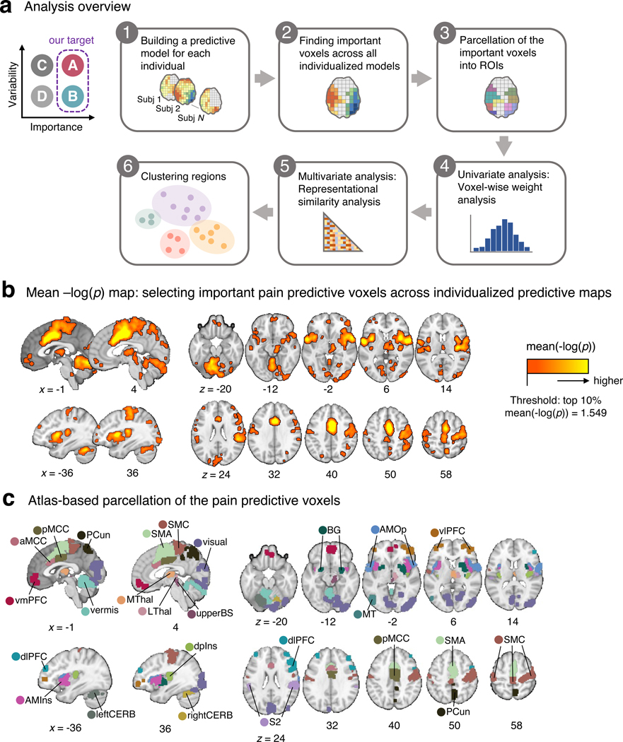
The current study encompasses two main objectives. First, we aimed to take a step toward personalized brain mapping of pain by employing idiographic predictive modeling. We trained a pain-predictive model for each individual from functional Magnetic Resonance Imaging (fMRI) data of 404 individuals from 13 single-trial thermal pain datasets collected by two independent laboratories. Among these, 11 datasets have been used in previous publications, and two datasets are unpublished (Supplementary Table 1). The second objective was to identify pain-predictive brain regions that show high versus low inter-individual variability in their pain representations. Previous studies mainly focused on brain regions that showed activation or deactivation patterns consistent across individuals. These studies, by design, could not identify brain regions that are important for pain processing but have idiosyncratic patterns (i.e., the “A” category in Fig. 1a). Thus, they provide an incomplete picture. To overcome this issue, we first identified pain-predictive brain regions based on their importance for within-individual pain prediction regardless of the between-individual consistency of the predictive weights (both “A” and “B” categories in Fig. 1a). We then quantified the inter-individual variability in regional weight patterns. We replicated our findings in an independent dataset (n = 124) and showed that they were not driven by variation in study-level task or acquisition parameters or varying signal quality across brain regions.

Figure 1. Analysis overview and important pain-predictive regions.

(a) In this study, we aimed to identify brain regions that were important for pain prediction and examine whether they showed variable or stable pattern representations across individuals (“A” and “B” categories; top left). To this end, we conducted a series of analyses that can be divided into six steps. Detailed explanations about the analysis steps can be found in the Results and Methods sections. (b) In the Step 2 analysis, we selected voxels that were important for pain prediction. We operationalized the importance in terms of mean –log(p), where the two-tailed p-values were calculated from the bootstrap tests performed in each individualized predictive map. The selected voxels had mean –log(p) values higher than the top 10% mean –log(p) value (= 1.549). (c) The important voxels were parcellated into 21 regions based on the cortical and cerebellar atlases (see Methods for more details).aMCC, anterior midcingulate cortex; AMIns, anterior middle insula; AMOp, anterior middle operculum; BG, basal ganglia; dlPFC, dorsal lateral prefrontal cortex; dpIns, dorsal posterior insula; leftCERB, left cerebellum; LThal, lateral thalamus; MT, middle temporal area; MThal, middle thalamus; PCun, precuneus; pMCC, posterior midcingulate cortex; rightCERB, right cerebellum; S2, secondary somatosensory cortex; SMA, supplementary motor area; SMC, sensorimotor cortex; upperBS, upper brainstem; visual, visual cortex; vlPFC, ventrolateral prefrontal cortex; vmPFC, ventromedial prefrontal cortex.

Together, we provide a comprehensive list of important pain-predictive brain regions and characterize them in terms of their inter-individual variability, elucidating which brain systems contribute to the inter-individual variability in pain processing. This study paves a path toward personalized brain mapping of pain and clinical interventions.

Results

Identifying brain regions important for pain prediction

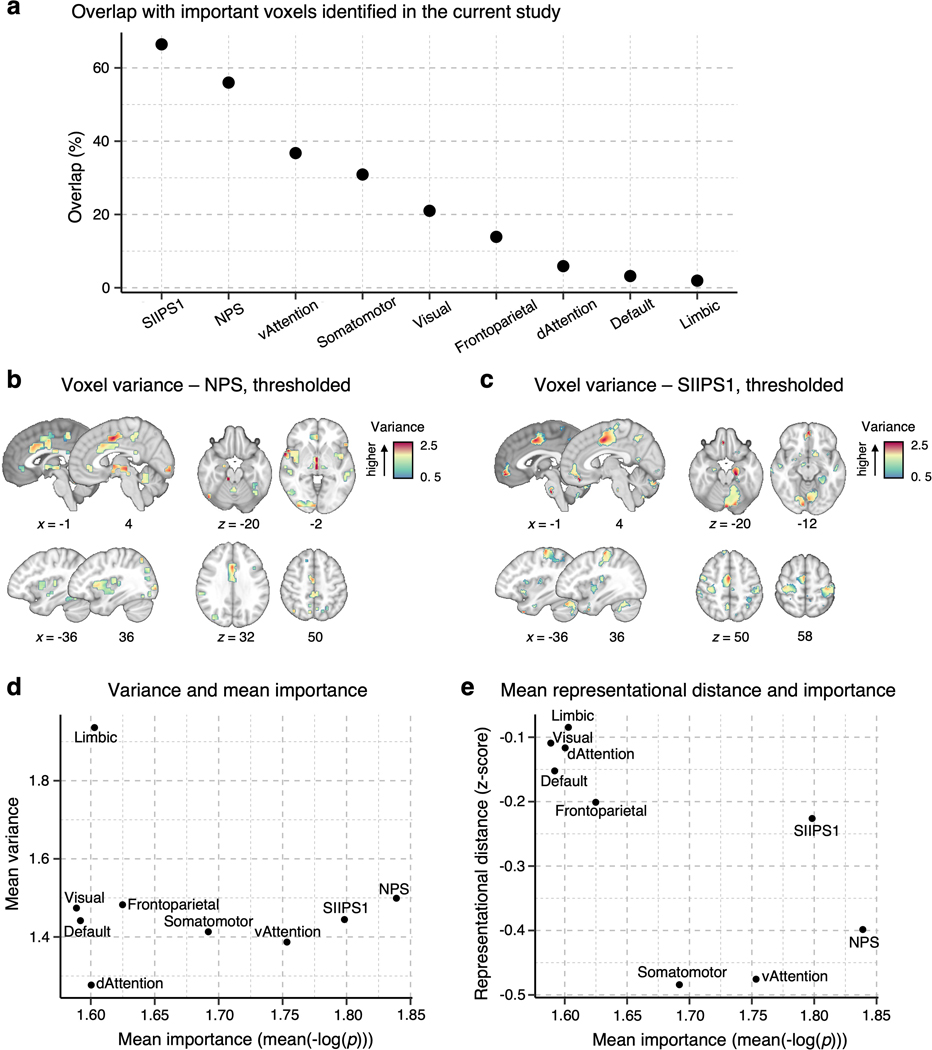
To find important pain-predictive brain regions (Analyses 1–3 in Fig. 1a), we fitted linear Support Vector Regression (SVR) models to data from each of the 404 participants in our dataset, creating 404 individualized pain-predictive maps (prediction-outcome correlation = 0.34 ± 0.01 [mean ± standard error of the mean] with 5-fold cross-validation), and identified important predictive features using bootstrap tests with 5,000 iterations for each predictive map. Unlike the population-level (or group-level) predictive modeling approach, which can identify only brain regions with multivariate pattern information consistent across individuals, our approach allows us to identify brain regions important for pain prediction within each individual even if the brain regions have distinct patterns across individuals. With the p-values from the bootstrap tests, we computed the mean –log(p) values for the whole brain across all individualized maps, and for further analyses we selected the top 10% voxels, of which the threshold was the mean –log(p) = 1.549. The selected voxels are displayed in Fig. 1b. We then parcellated the voxels into regions based on multiple anatomical atlases, identifying 21 regions as important for pain prediction (Fig. 1c). For further reference to other commonly used parcellations and brain signatures of pain, we calculated the overlap of the Neurologic Pain Signature¹⁷ (NPS), Stimulus Intensity Independent Pain Signature-1¹⁹ (SIIPS1), and large-scale resting-state functional networks²⁰ with the selected voxels. We found larger overlap with our regions in SIIPS1, NPS, ventral attention and somatomotor networks than other networks (Extended Data Fig. 1a). Additionally, a preliminary analysis, in which we compared the prediction performance of individualized models and group-based models on three-session data from a single individual and data from Study 14, suggested that individualized models achieve higher prediction accuracy than group-based models (Supplementary Fig. 1).

The 21 pain-predictive regions included (in alphabetical order), the 1) anterior midcingulate cortex (aMCC), 2) anterior middle insula (AMIns), 3) anterior middle operculum (AMOp), 4) basal ganglia (BG), 5) dorsal lateral prefrontal cortex (dlPFC), 6) dorsal posterior insula (dpIns), 7) left cerebellum (leftCERB), 8) lateral thalamus (LThal), 9) middle temporal area (MT), 10) middle thalamus (MThal), 11) precuneus (PCun), 12) posterior midcingulate cortex (pMCC), 13) right cerebellum (rightCERB), 14) secondary somatosensory cortex (S2), 15) supplementary motor area (SMA), 16) sensorimotor cortex (SMC), 17) upper brainstem (upperBS), 18) vermis, 19) visual cortex (visual), 20) ventrolateral prefrontal cortex (vlPFC), and 21) ventromedial prefrontal cortex (vmPFC). We applied masks of these regions to the individualized predictive maps and used only the masked voxel data for further analyses. The individualized maps, region masks and other data and code are available at https://github.com/cocoanlab/individual_var_pain.

Univariate analysis of the individual variability

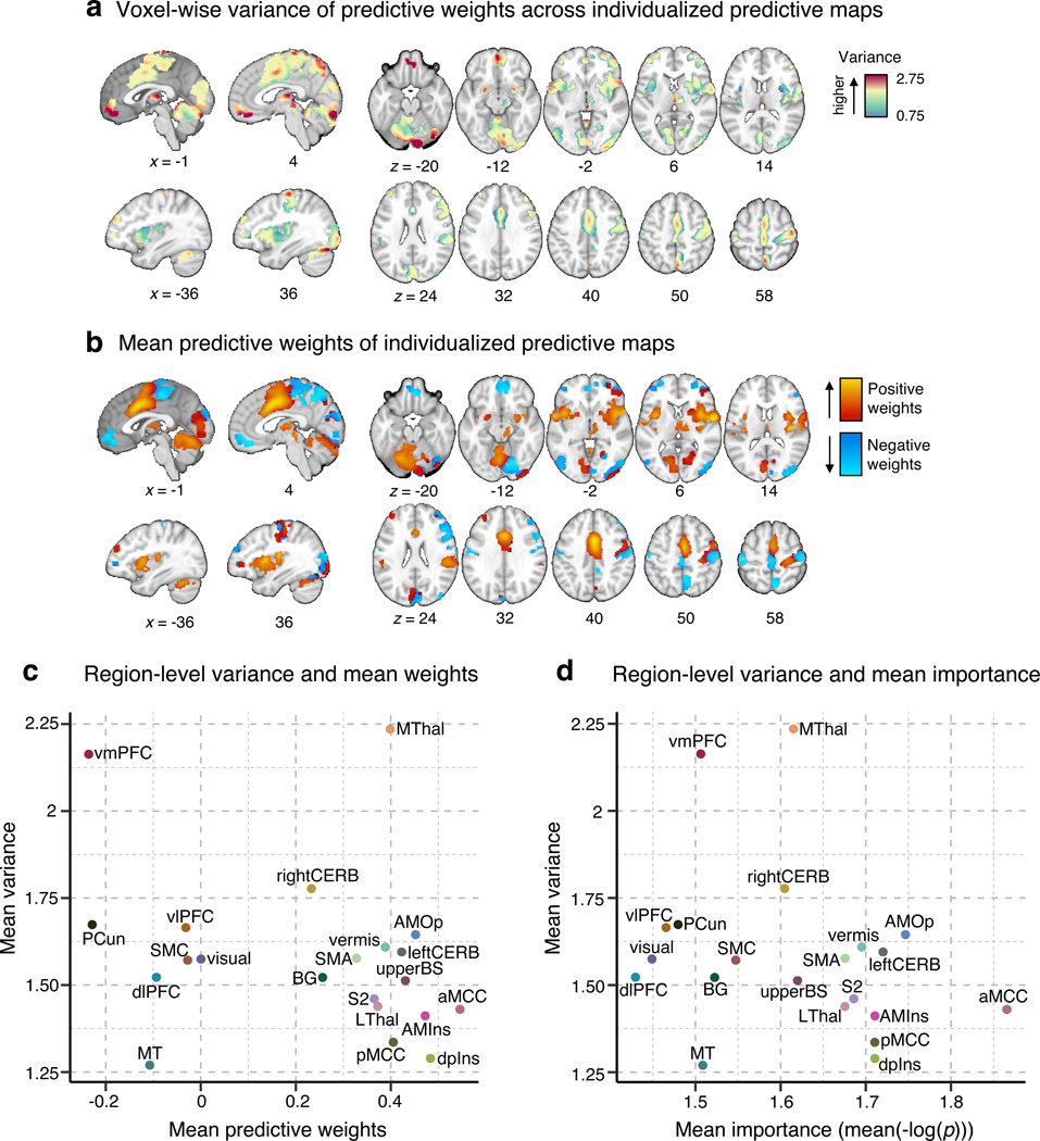
We first examined the voxel-wise individual variability of the predictive weights for the important pain-predictive regions using variance across all individualized maps (Analysis 4). Before calculating the voxel-wise variance, we normalized each predictive map by dividing the weights by the spatial standard deviation across the whole brain, rendering their scales comparable across images. The variance of the individual voxel weights is visualized in Fig. 2a. The region-level summary shown in Fig. 2c indicates that the vmPFC and MThal showed relatively high weight variance, while the MT, dpIns, and pMCC showed low weight variance. For additional reference, we examined the voxel-wise variance in the large-scale resting-state functional networks²⁰, NPS¹⁷, and SIIPS1¹⁹, finding the highest variance in the limbic network and the lowest variance in the dorsal attention network (Extended Data Fig. 1d).

Figure 2. Univariate analysis of the individual variability of predictive weights.

(a) We first examined the voxel-wise variance of voxel weights across all individualized pain-predictive maps. (b) We also examined the voxel-level mean predictive weights across the individualized maps. The positive weights were shown in warm colors (i.e., positively predictive of pain), and the negative weights (i.e., negatively predictive of pain) were shown in cool colors. (c) The scatter plot shows the region-level summary with the mean predictive weights on the x-axis and mean weight variance on the y-axis. (d) The scatter plot displays the mean weight variance against the mean importance as –log(p) (based on two-tailed p-values).

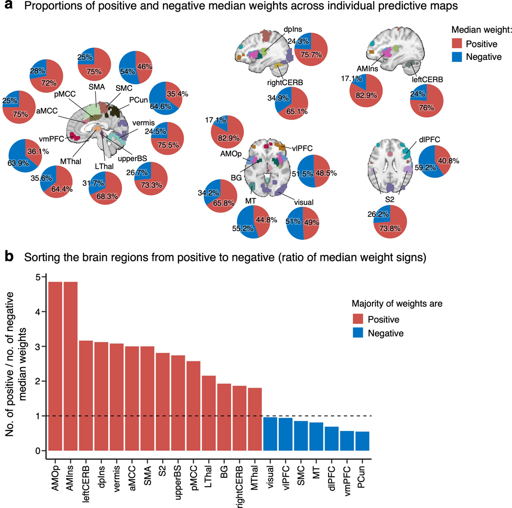
The signs of averaged voxel weights were largely consistent with those in previous literature. For example, brain regions such as the insula, S2, MCC, and thalamus were, on average, positively predictive of pain, while the prefrontal cortices and PCun were negatively predictive (Fig. 2b,c)^17,19. This result may seem to suggest that the brain regions have consistent roles in pain prediction across people. However, when examining the signs of median voxel weights in individuals, we found a large individual variability as the proportion of positive versus negative signs across people, indicating that regions were not strictly positive or negative in all subjects (Extended Data Fig. 2a). For example, the vmPFC consisted of negative weights on average, but 36.1% of the subject median weights were positive, indicating variability in the sign of the multivariate pattern. Similarly, the dlPFC, MT, PCun, and vlPFC showed negative average weights, but their median weights were positive in 40.8%, 44.8%, 35.4%, and 48.5% of individuals, respectively. The most variable weight sign appeared in the visual cortex with 49% positive and 51% negative median weights (Extended Data Fig. 2b). This indicates substantial individual variability in the functional role and/or functional topography in relation to pain in these areas. Fig. 2d depicts the relationship between the region-level variance and region importance.

Multivariate analysis of the individual variability

Although the univariate approach can provide useful voxel-level information about the individual variability of predictive weights, the multivariate patterns may convey more critical information about neural population codes of pain processing for each individual^17,21. Additionally, multivariate analyses have been shown to be more stable and less influenced by noise than univariate approaches²². Therefore, as a next step, we assessed the variability of the regional multivariate patterns across individuals using representational similarity analysis²³, which allowed us to quantify the similarity between the spatial patterns of corresponding regions across different individuals (Analysis 5).

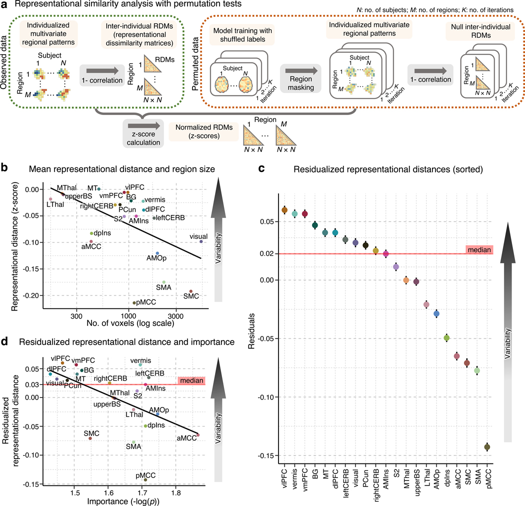
As shown in Fig. 3a, we first calculated the inter-individual representational dissimilarity matrices (RDMs) as a measure of the inter-individual distance for the 21 pain-predictive regions using regional multivariate pattern information extracted from the 404 individualized pain-predictive maps (from 404 participants), resulting in 21 404-by-404 RDMs. To ensure fair comparisons among different regions that have different locations and sizes, we normalized the RDMs (i.e., obtained z-scores) using null RDM baselines for each region resulting from a permutation test (see Methods for more details).

Figure 3. Multivariate analysis of the individual variability of predictive weights using a representational similarity analysis.

(a) To assess the inter-individual variability of the regional multivariate patterns, we performed a representational similarity analysis²³. A detailed description of the analysis can be found in the Methods section, Multivariate representational similarity analysis. (b) The scatter plot shows the relationship between the mean representational distance based on the permutation tests (y-axis) and region size (displayed in the logarithmic scale on the x-axis). The two variables showed strong negative correlation, r = −0.537, p = 0.012, two-tailed. Higher representational distance values indicate higher pattern-level variability across people. (c) To account for the effects of region size on the representational distance, we regressed out the region size effects from the representational distance. The plot shows the residualized representational distance, sorted from the highest distance, and the standard error of the mean across all pair comparisons of individuals, i.e., C(404, 2) = 81,406. (d) The scatter plot shows the relationship between the residualized representational distance and the mean importance measured by mean -log(p) with Pearson’s r = –0.542, p = 0.011, two-tailed.

Fig. 3b displays the averages of the lower triangles of the normalized RMDs (i.e., mean z-scores) against the number of voxels of the pain-predictive regions, suggesting a strong negative linear relationship between the mean representational distance and region size even after the permutation-based normalization (Pearson’s r = –0.537, p = 0.012). Thus, to further account for the effects of region size, we regressed out the effects from the mean representational distances. The residualized mean representational distance for each region is displayed in Fig. 3c, indicating that the vlPFC, vermis, and vmPFC showed the highest individual variability while the pMCC, SMA and SMC appeared to be the most stable across individuals. Additional results without residualizing the region size are shown in Supplementary Fig. 2. For further reference, we performed the analysis in the NPS¹⁷, SIIPS1¹⁹, and large-scale functional networks²⁰. The limbic and visual networks manifested the highest inter-individual variability, whereas the somatomotor and ventral attention networks and NPS showed the lowest variability (Extended Data Fig. 1e). Lastly, Fig. 3d shows the relationship between the residualized mean distance and mean importance (the mean –log(p) values) of each region with Pearson’s r = –0.542, p = 0.011, suggesting that highly important regions for individualized pain prediction also have more stable multivariate patterns across people.

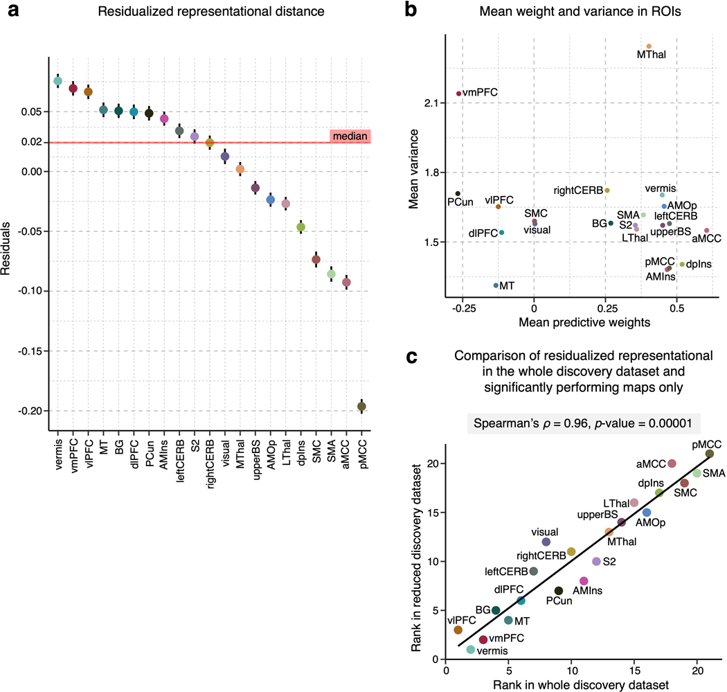
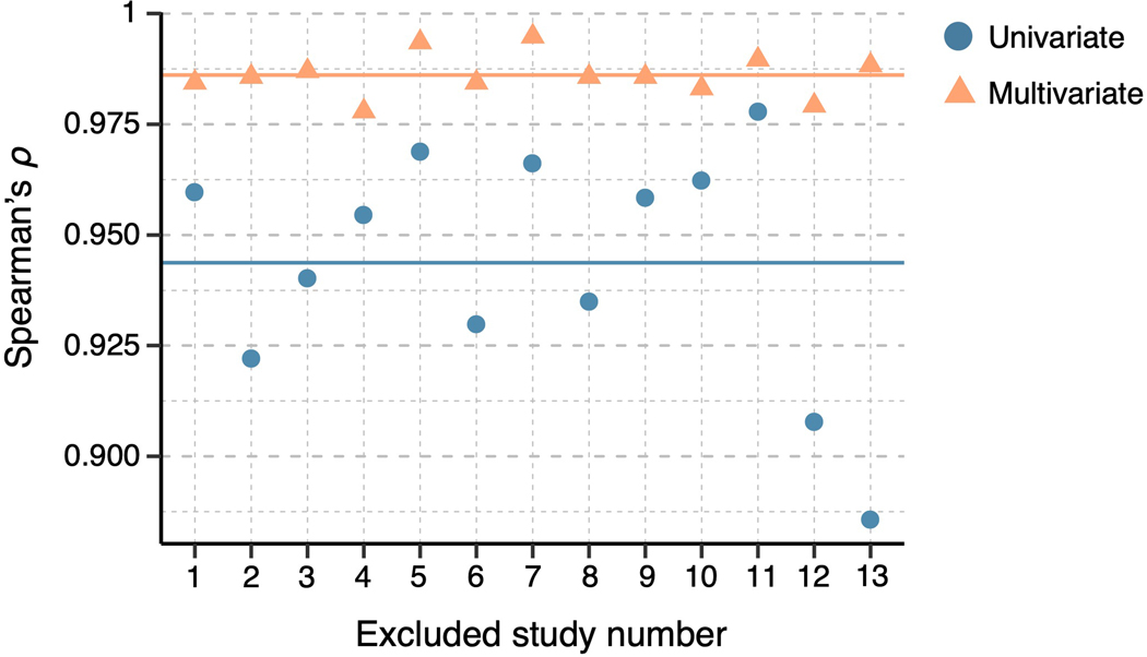
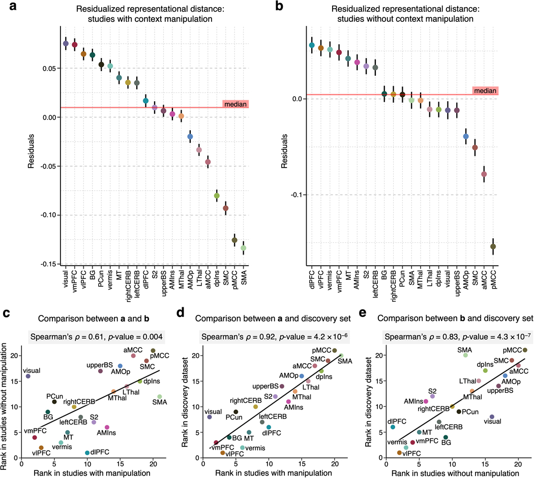
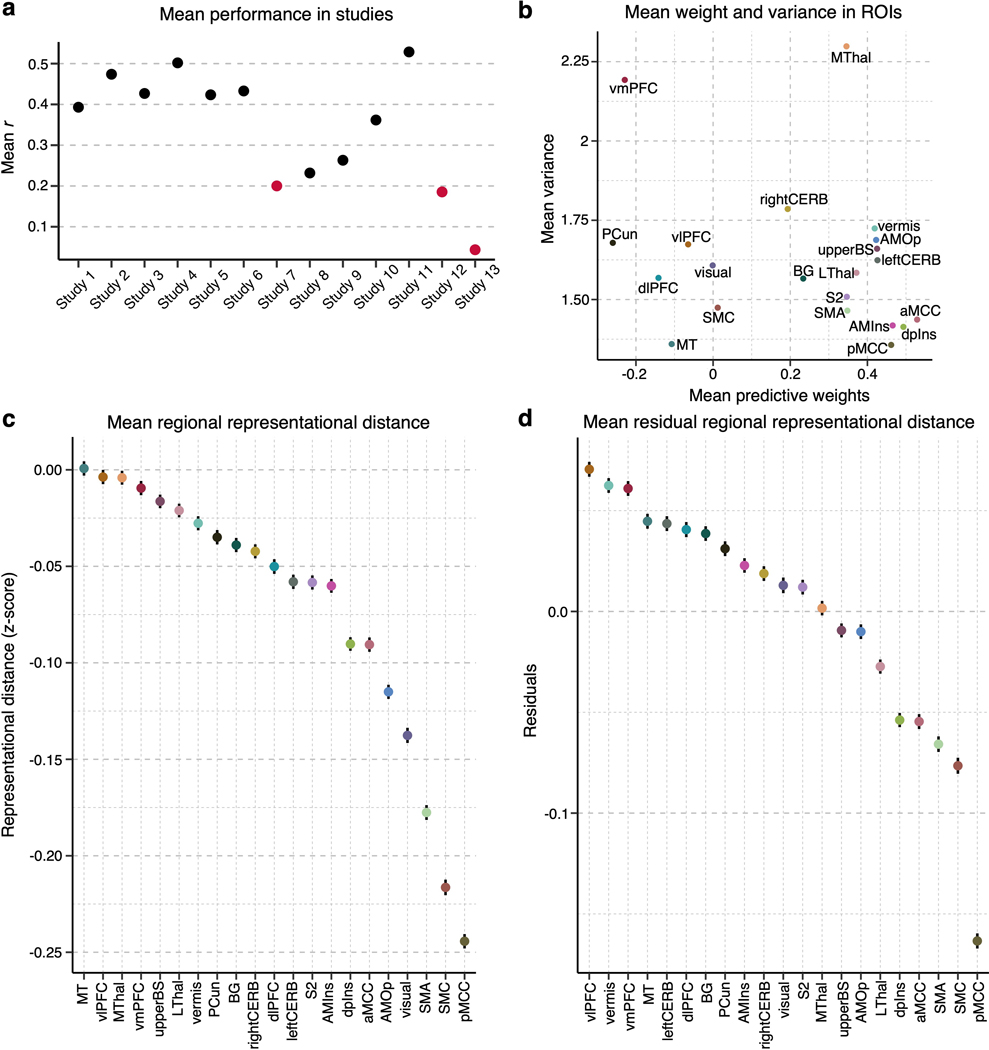
We performed several analyses to assess the robustness of the results. Results from analyses run on a reduced dataset of individualized models with significant prediction performance only were significantly correlated with the results based on the full dataset at Spearman’s ρ = 0.96, p = 0.00001. (Extended Data Fig. 3). We additionally tested whether each study had a significant effect on the final results (i.e., the variability ranking among 21 regions) by removing one study from all analyses at a time (i.e., a study-level jackknife), repeating this whole analysis for all 13 studies, and comparing the results of a reduced set of studies with the original results of the full set of studies. Both the univariate and multivariate analyses showed stable results even after removing each study. Spearman’s correlation coefficient ranged from 0.86 to 0.98 for the univariate results and from 0.98 to 0.99 for the multivariate results (Extended Data Fig. 4), suggesting that each study and study-specific parameters had minimal effects on the results. We also tested the effects of context manipulations present in some studies in our dataset, such as placebo or cognitive regulation. To assess the impact of these manipulations, we performed the representational similarity analysis separately on subsets of studies with and without context manipulations. Results from studies with and without context manipulation were significantly correlated with the results based on the whole dataset with Spearman’s ρ = 0.92, p = 4.2 × 10⁻⁶, and ρ = 0.83, p = 4.3 × 10⁻⁷, respectively (Extended Data Fig. 5). Additionally, we investigated the effects of study-related variables on the inter-individual variability within regions. We performed a multiple regression analysis with independent variables (x-variables) being study-related factors such as the field strength of the scanner, data collection site, stimulated body site, stimulus duration, number of trials available for the participant, and presence of pain predictive cues, with the dependent variable (y-variable) being the mean inter-individual distance in each region of interest (Supplementary Table 2). Although some regression models showed sensible significant effects of some variables, the main findings presented here were not affected after controlling for these effects (Spearman’s ρ = 1.0) as the analysis was conducted within each region and our main findings compared the inter-individual variability across regions. Finally, we tested whether the pattern of results was influenced by excluding studies with low within-study prediction performance. We performed the analyses excluding three studies with the lowest average prediction performance and found that the overall pattern of results presented here was preserved (Extended Data Fig. 6). Thus, in sum, the results are robust across studies that vary in psychological context and not driven by individual studies or studies with poorer overall prediction performance.

Replication in a large-scale independent dataset

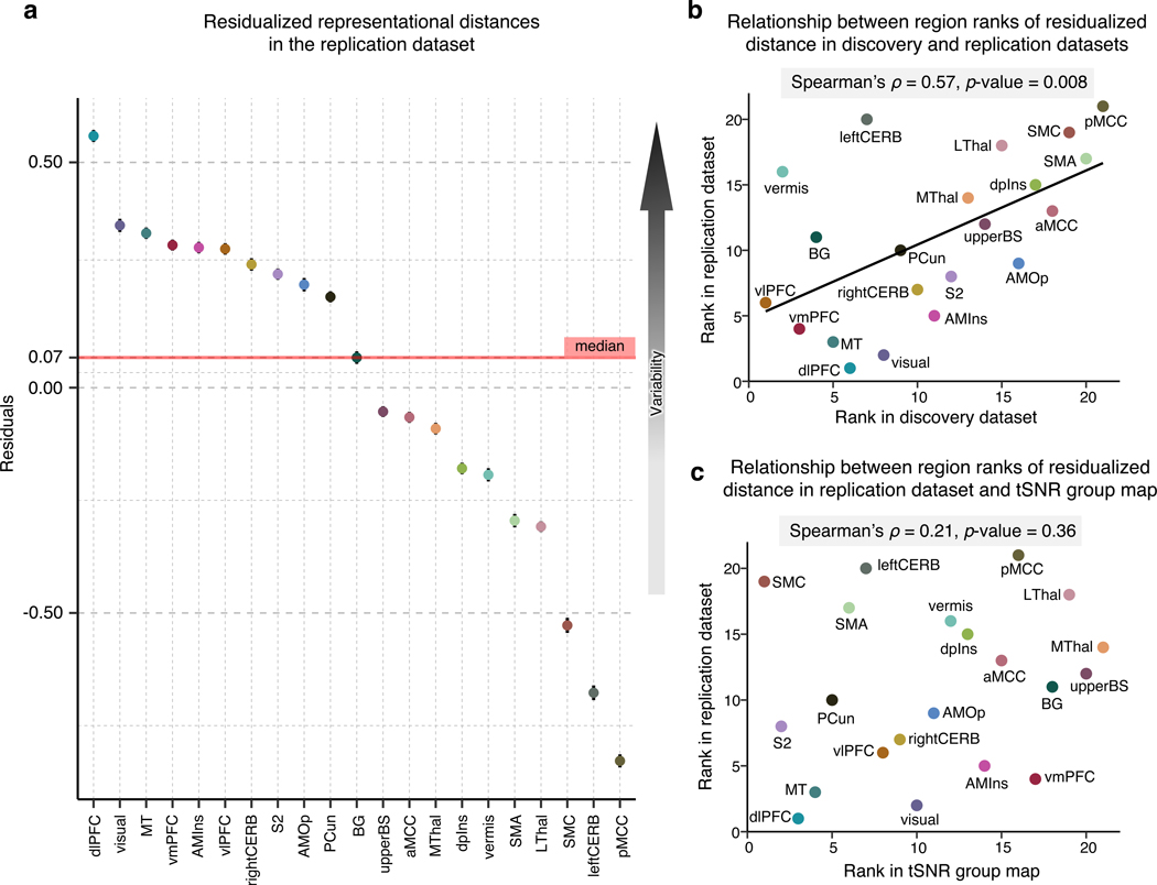
To further validate and show that our findings are not a mere consequence of different experimental designs across multiple studies and varying signal quality across brain regions, we replicated our findings with a large-scale independent dataset (n = 124) acquired at one location with a single experimental design. As in the discovery dataset, we fitted an SVR model to the single-trial data and obtained 124 individualized predictive maps (prediction-outcome correlation = 0.68 ± 0.02, mean squared error = 0.014 ± 0.001 with 5-fold cross-validation). We then applied the region masks, performed a multivariate representational similarity analysis on the masked regional data, and regressed out the effects of region size on the mean representational distance. Fig. 4a shows the residualized distance indicating that the highest inter-individual variability was found in the dlPFC, visual areas, and vmPFC, while the pMCC, leftCERB and SMC manifested the lowest variability. To compare this result with the result from the discovery dataset, we assigned a rank to each region based on the residualized distance in both datasets and measured the rank correlation between them. The rank correlation coefficient, Spearman’s ρ, was significant at a value of 0.57, p = 0.008 (Fig. 4b). We also evaluated whether the important pain-predictive voxels identified in the discovery dataset also replicate in this replication dataset. We found a significant phi correlation, ɸ = 0.502, p < 2.2 × 10⁻¹⁶, suggesting high similarity between the two binarized voxel importance maps (Supplementary Fig. 3). Additionally, we performed a preliminary test of within-individual reliability of the predictive patterns by splitting the data for each individual into two folds (i.e., the first four and the last four runs), training models on both folds and evaluating the similarity of the whole-brain and regional predictive patterns. The pattern similarity showed mostly medium to large correlations, providing preliminary evidence of within-individual reliability of the predictive patterns (Supplementary Fig. 4a). We also performed the same analysis on a preliminary four-session dataset from a single participant, obtaining further support for within-individual reliability (Supplementary Fig. 4d).

Figure 4. Replication of the multivariate representational similarity analysis in an independent dataset and tSNR in the dataset.

To validate the previous results, we employed an independent replication dataset acquired under the same experimental settings in the same location. (a) In the replication dataset, we performed a representational similarity analysis and regressed out the effects of region size on the mean representational distance. The plot depicts the residualized representational distance (a measure of inter-individual variability in neural patterns) in each region, with higher values representing higher regional variability. (b) Based on the residualized distance, we assigned ranks to all regions in both the discovery and replication datasets. The scatterplot visualizes the statistically significant relationship between the results in the two datasets. (c) To further inspect whether our results in the replication dataset are influenced by a different tSNR in different regions, we calculated the mean tSNR in all regions. The scatter plot compares the region ranks based on the tSNR and residualized representational distance suggesting that the regional variability in the replication dataset cannot be explained by varying tSNR in regions.

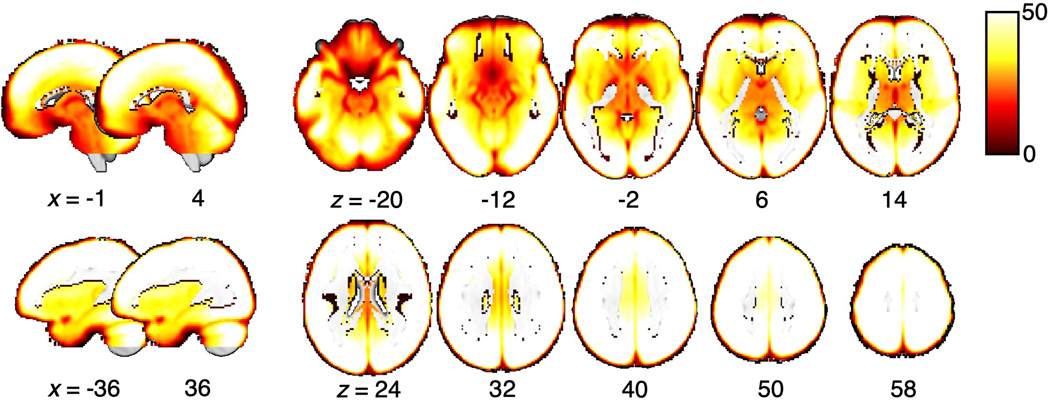
Since the signal quality in the fMRI data may vary across brain regions, which in turn may affect the regional variability, we examined whether the temporal signal-to-noise ratio (tSNR) of our data is correlated with our results. To this end, we first calculated the tSNR for each participant as the mean of images acquired at each repetition time (TR) divided by the standard deviation. Subsequently, we obtained a group-average tSNR map (Extended Data Fig. 7) and calculated the mean tSNR for each region. We then assigned ranks to regions based on the tSNR and compared them with the ranks based on the residualized representational distance using rank correlation. The comparison suggested that the regional variability cannot be explained by varying tSNR across regions (Spearman’s ρ = 0.21, p = 0.36; Fig. 4c).

Clustering pain-predictive brain regions

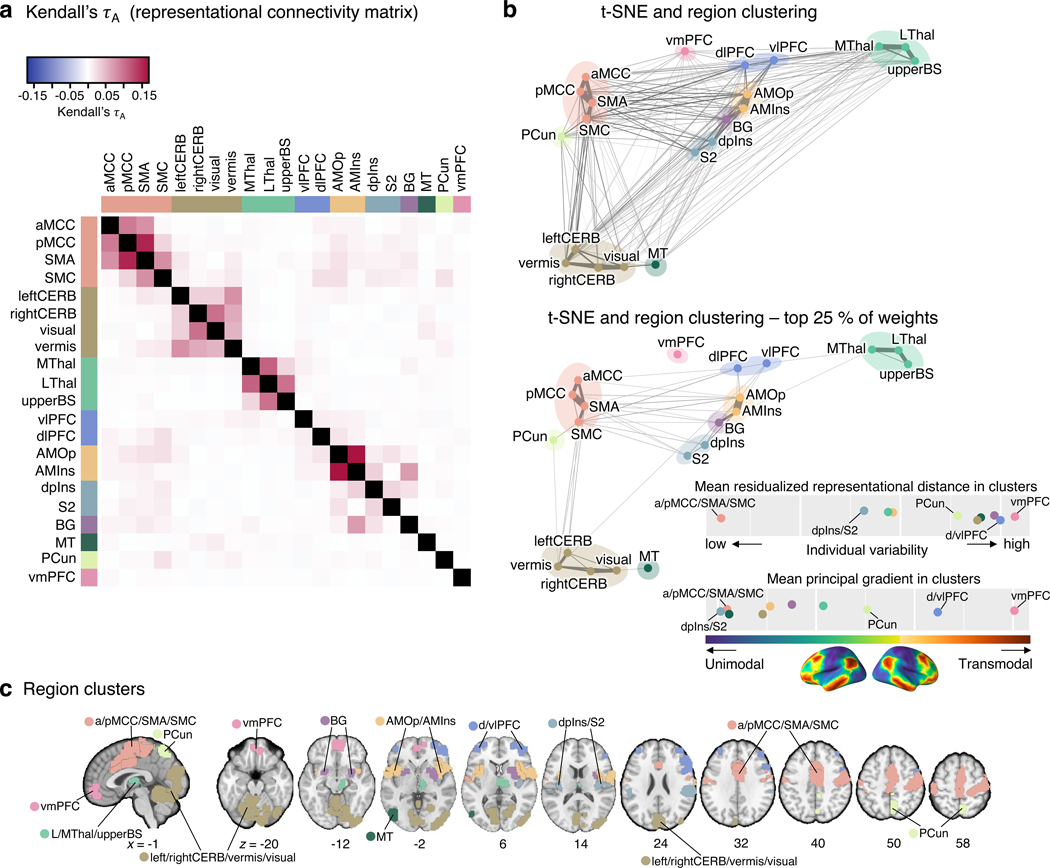
Next, we compared the regional inter-individual variability profiles using non-parametric rank correlation Kendall’s τ_A to identify clusters of brain regions that exhibited similar patterns of the representational distance across individuals (Analysis 6). This correlation matrix provides the representational connectivity (as termed by Kriegeskorte et al.²³) among 21 pain-predictive regions, which quantifies the representational information shared across regions. This approach can be regarded as a type of multivariate connectivity that allows us to group multivariate pattern representations using clustering analysis. The Kendall’s τ_A values ranged from –0.005 to 0.17 (Fig. 5a), with higher values indicating higher similarity in the individual variability patterns for a pair of regions. For example, relatively high similarity was found between the AMOp and AMins with Kendall’s τ_A of 0.17, between the SMA and pMCC with the value of 0.155, or between the MThal and LThal with the value equal to 0.112.

Figure 5. Clustering of the pain-predictive brain regions based on the patterns of representational distance.

(a) The heat map shows the representational connectivity matrix (Kendall’s τ_A) among 21 pain-predictive regions. Higher Kendall’s τ_A values (shown in darker red) indicate higher similarity between regions. (b) We conducted a hierarchical clustering analysis of brain regions using the 10-dimensional NMDS scores based on the representational connectivity matrix, resulting in 10 region clusters. The plot shows the t-distributed stochastic neighborhood embedding (t-SNE) map based on the 10-dimensional NMDS scores, and the 10 region clusters are shown with different colors. The line widths indicate the relative connectivity strengths among the brain regions. The top panel shows all the connections, while the bottom panel shows only the top 25 % of the connections. The upper bottom right chart displays the mean residualized representational distance of the region clusters (color-coded). Furthermore, in the region clusters we calculated the mean principal gradient that ranges from unimodal to higher-order transmodal areas as suggested by ref.²⁴. The lower chart, then, shows the mean principal gradient in the region clusters suggesting that more variable clusters are located at the top of the principal gradient spectrum, while more stable clusters are located at the bottom of the principal gradient. The bottom cortex map visualizes the principal gradient map obtained from an independent dataset (N = 59). (c) The region clusters are visualized on a brain underlay.

To cluster the 21 pain-predictive regions based on the patterns of inter-individual representational similarity, we first transformed the Kendall’s τ_A into a distance matrix and performed nonmetric multidimensional scaling (NMDS). NMDS scores were then used as input features for hierarchical clustering. To select the optimal number of clusters (k), we compared the clustering quality scores (silhouette values) against the null-hypothesis baseline obtained from a permutation test for k = 2 to 15 solutions (see Methods for details). The optimal k was 10 clusters, which performed at the mean silhouette score of 0.59 (from the range of 0 to 1, where 1 indicates perfect separability of clusters) with z = 3.72, p = 0.0002 over the null baseline clustering quality (for more details, see Extended Data Fig. 8). The identified clusters of regions included the aMCC, pMCC, SMA, and SMC for cluster 1; the leftCERB, rightCERB, vermis, and visual cortex for cluster 2; the dpIns, and S2 for cluster 3; the AMIns, and AMOp for cluster 4; the vlPFC and dlPFC for cluster 5; and the MThal, LThal, and upperBS for cluster 6. Also, the BG, MT, PCun and vmPFC each constituted a standalone cluster.

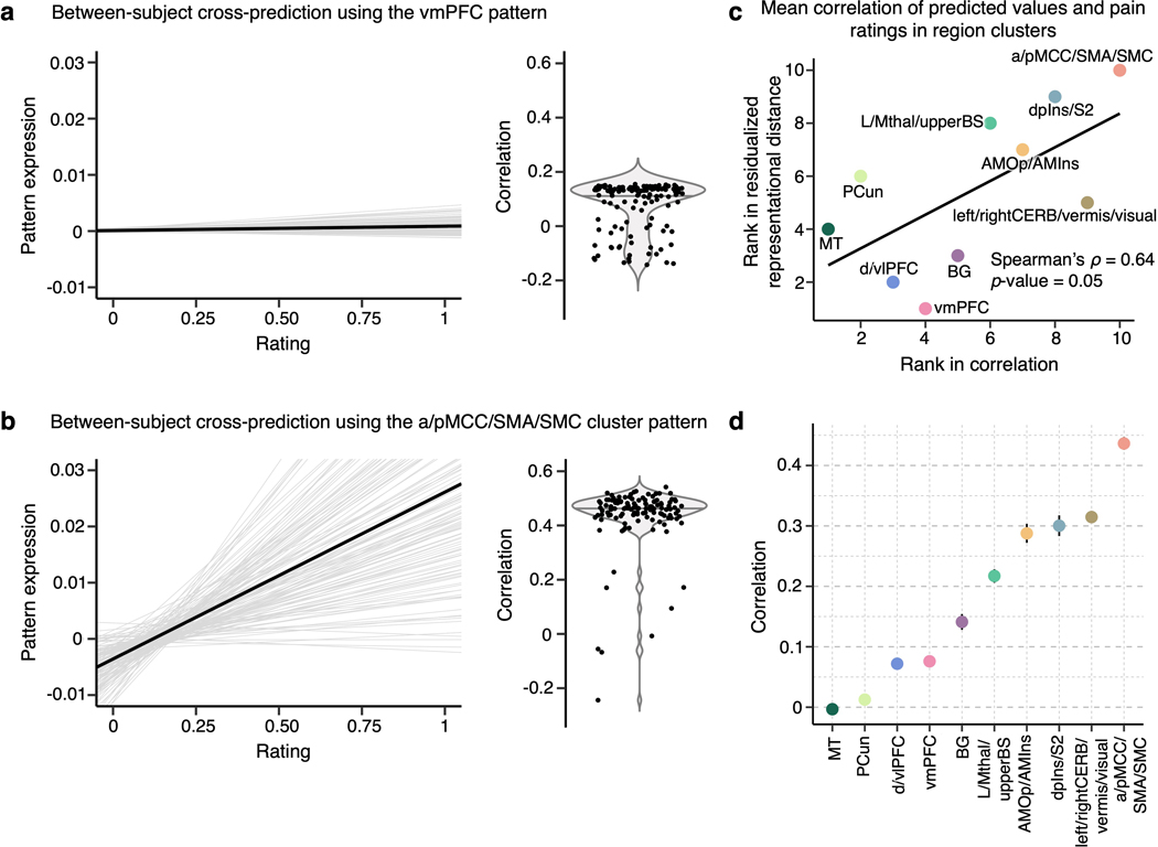
For display, we performed t-distributed Stochastic Neighborhood Embedding (t-SNE) on the NMDS scores and plotted it with Kendall’s τ_A values transformed into weights connecting the regions in color-coded region clusters (Fig. 5b). With thresholding to show only the top 25% of connection weights, the vmPFC was not connected to any other region, suggesting that the vmPFC showed a unique pattern of individual variability of predictive weights distinct from other brain regions (bottom panel of Fig. 5b). After computing the mean residualized representational distance of the clusters, the vmPFC and d/vlPFC clusters showed the highest distance among the region clusters, and the aMCC/pMCC/SMA/SMC and S2/dpIns clusters showed the lowest distance among the clusters (Fig. 5b). For further illustration of the inter-individual variability in the region clusters, we applied the predictive patterns of the region clusters from each individual to the activation maps of all other individuals to predict the corresponding pain ratings (Extended Data Fig. 9). The results show that the cross-individual prediction performance is correlated with the inter-individual variability of the clusters, with the cross-individual prediction being more reliable in the less variable clusters. In other words, along with our results in Supplementary Fig. 4 where we showed that predictive weights are reliable within individuals, these results support the idea that the inter-individual variability of the regional predictive weight patterns is driven by individual variability in brain representations of pain, not by mere degeneracy properties common in high-dimensional data modelling or noise.

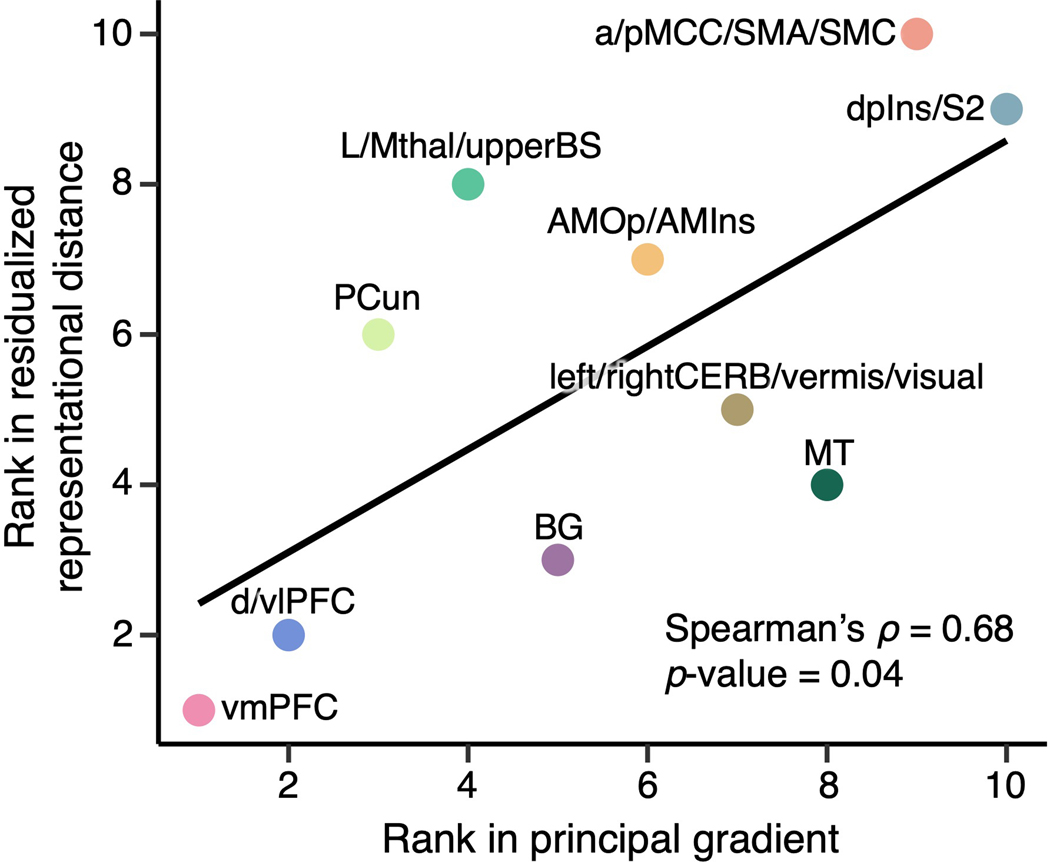
We also explored the relationship between these clusters and cortical hierarchy levels identified using unimodal-to-transmodal connectivity gradients²⁴. Here, the principal connectivity gradient captures the diversity of functional connectivity patterns on a spectrum ranging from unimodal to higher-order transmodal brain structures²⁴. We calculated the mean principal gradient in our region clusters based on a principal gradient map derived from an independent resting-state fMRI dataset (N = 59). The results showed that the mean residualized distances were significantly correlated with the mean principal gradients (Spearman’s ρ = 0.68, p = 0.04; Extended Data Fig. 10), suggesting that the areas in which pain representations are more variable across individuals are higher-order transmodal regions located at the top of the principal gradient, while those that are stable across individuals are unimodal sensory regions located at the bottom of the cortical hierarchy.

Discussion

Our study investigated the heterogeneity of individualized brain representations of pain based on fMRI data from a large sample of n = 404 for discovery and n = 124 for replication (total N = 528). Across all individualized pain-predictive maps, we first identified 21 predictive regions. Among these, the prefrontal and cerebellar regions, including the vmPFC, vlPFC, dlPFC, vermis, and leftCERB, showed high inter-individual variability in both univariate and multivariate analyses. In contrast, the cingulate, somatomotor, and insular cortices, including the a/pMCC, SMA, SMC, and dpINS, showed lower inter-individual variability. Importantly, this finding was successfully replicated in an independent dataset of n = 124, demonstrating (along with multiple supplementary analyses) that the pattern heterogeneity was not a mere effect of various experimental settings or noise. Clustering regions based on inter-personal representational distance in multivariate predictive patterns revealed 10 groups of regions, with more inter-personally variable groups lying on the transmodal end of the spectrum of the principal gradient of cortical organization and more stable groups on the unimodal end. Overall, the current study aims to step toward individualized pain brain mapping by providing brain targets that hold the potential to be a basis for further development of individualized clinical interventions and brain-based subtyping of individuals in pain representations.

Most of the important pain-predictive brain regions identified here have also been reported in previous studies (see refs.^3,4). Additionally, the signs of group-level predictive weights (i.e., whether a brain region is positively or negatively correlated with pain ratings) were largely consistent with previous studies that used experimental acute pain stimuli^25,26. However, we also found large individual variability in the predictive weight signs of the individualized pain-predictive maps (e.g., Extended Data Fig. 2), suggesting that each region’s functional role in pain processing varies across individuals. Therefore, our findings indicate that the individualized functional relationships between brain regions and pain perception are more complicated than how they are usually summarized at the group level. Although group-level summaries certainly have their own merits and strengths, such as canceling out noise and identifying findings that are most reproducible across individuals, the idiosyncratic patterns of pain-predictive weights that will be crucial to understanding the personal pain experience are often ignored. However, our approach allowed each individualized pain-predictive map to have different signs and patterns of weights by focusing on group-level averages of the “importance” measure. For example, the visual cortex regions might not often appear in pain neuroimaging studies, perhaps because of its mixed relationship with pain perception, as shown in Extended Data Fig. 2. However, our results suggest that the visual cortex is also an important contributor to pain prediction consistently across people. The functional role of the visual cortex could be manifold, for example, multisensory integration²⁷, task-related²⁸, or enhanced attentional state as a consequence of a salient event²⁹.

Combining results from both the univariate and multivariate analyses, we found that the brain regions that showed stable patterns across individuals were mostly those receiving direct inputs from the spinothalamic pathways, including the MCC (aMCC and pMCC), SMC, SMA, and insula (dpIns and AMIns)^30,31. In contrast, the brain regions that showed variable patterns across individuals were the prefrontal and cerebellar regions, including the vlPFC, vmPFC, vermis, and rightCERB. Among these regions, the MCC appeared to have the most stable predictive weights in both the univariate and multivariate analysis results. The MCC is known to work as a hub for processing of the affective-motivational components of pain and behavioral control of pain-related responses^32,33. In particular, the MCC receives direct inputs from the medial thalamus³⁰, and it has been recognized as a part of the medial pain pathway, which has been associated with processing of the affective-motivational component of pain³⁴. However, whether the medial pathway is specialized in processing this particular pain component has been challenged³³. It has also been shown that the MCC contains neurons responding specifically to nociception³⁵, and exhibits generalizable multivariate pain-specific representations³⁶. Another brain region with a stable representation across individuals was the dpIns, which is among the regions that best track the perceived intensity of pain³⁷ and are most consistently reported in pain neuroimaging studies³⁸. Supporting the role of the dpIns in nociception, research in monkeys has revealed direct nociceptive-specific projections from the spinothalamic system to the posterior part of the insula encoding modality, location, and intensity of the incoming stimulus³⁹.

On the other hand, the vlPFC and vmPFC had the most variable representations across individuals. These brain regions are known to be important for cognitive pain modulation, such as reappraisal and placebo^40,41 and pain catastrophizing⁴². In particular, the vmPFC is important for autobiographical memory representations, valuation⁴³, and endogenous cognitive and affective processes^44,45, supporting the possibility that these prefrontal regions subserve individually unique representations of pain. High between-study variability in frontal areas, likely stemming from different study contexts, was also reported in a recent meta-analysis on placebo analgesia⁴⁶. In addition to the prefrontal regions, striatal and cerebellar regions also showed variable representations across individuals. Given that the cerebellar contributions to pain have only recently become of interest⁴⁷, further research will be required to fully understand our findings in the cerebellum.

Importantly, these findings were replicated using an independent dataset. Unlike the discovery dataset, the replication dataset was collected under a single experimental setting; thus, it provided an appropriate basis to test whether the idiosyncrasy is a mere effect of the heterogeneity of the discovery dataset or reflects actual characteristics of the regions. Along with the evidence that the regional tSNR is not related to individual variability, study-level jackknife, and other supplementary analyses, the replication results provide supporting evidence for our findings in the discovery set.

There was also a slight discrepancy between the results of the univariate and multivariate analyses. In particular, the MThal had the most variable representation in the univariate analysis, whereas it was below the median (i.e., less variable) in the multivariate analysis. Additionally, the MT was stable in the univariate analysis, but more variable in the multivariate analysis. These discrepancies may stem from the different nature of the analyses. The univariate analysis considers individual voxels separately and, therefore, becomes more vulnerable to outliers. However, the multivariate analysis considers the whole pattern of voxel activations and thus should be more stable than the univariate analysis and capture representational features lost in the univariate analysis.

We also identified 10 region clusters based on the patterns of inter-individual variability. The region clusters were mostly composed of regions that are anatomically and functionally adjacent, e.g., S2 and dpIns, thalamus and brainstem. However, the vmPFC, PCun, MT and BG each constituted a standalone cluster, which may reflect their high individual variability and unique representations of pain. Interestingly, we also observed a relationship between the inter-individual variability of the clusters and the principal gradient of cortical organization based on functional connectivity patterns²⁴. The gradient spans from unimodal sensory cortical regions that process concrete direct percepts to higher-level transmodal regions that integrate and process abstract information⁴⁸. Along with this notion, region clusters with lower inter-individual variability were found in the unimodal end of the gradient spectrum, including dpIns/S2 and aMCC/pMCC/SMA/SMC clusters that receive direct spinothalamic nociceptive inputs. Many of these (particularly dpIns and S2) are unimodal in that they are highly selective for somatosensory input or even nociceptive input (as with dpIns) more specifically. On the other hand, region clusters that showed higher variability, such as vmPFC, dlPFC/vlPFC, or PCun clusters, were in the transmodal end of the spectrum, suggesting that regions in the higher end of the cortical hierarchy show more individual-specific representations. Interestingly, this finding is consistent with Finn et al.⁴⁹ in which the higher-level transmodal regions including the frontoparietal and default mode networks were best performing at identifying functional connectivity fingerprints.

The region clusters provided here hold a potential to be, ultimately, used as targets for brain-based biotyping for pain or personalized clinical interventions. Interest in precision medicine and individualized brain mapping has recently increased^14,15,49 because such individualized approaches could potentially improve the effects of treatment by tailoring it to the needs of each individual and provide evidence for disease subtypes. Therefore, as an example benefit of our approach, knowing which brain regions are important for pain processing and whether their pain representations are variable or consistent across individuals could help in making decisions about the deep brain stimulation or transcranial magnetic stimulation locations for chronic pain treatment^50,51. The knowledge of which regions show high or low inter-individual variability could also be useful for biomarker development and decoded neurofeedback^1,52. As the outcomes of regions with different levels of inter-individual variability could vary, these strategies could be informed of which brain regions could be more reliable targets across a population and which are better suited for personalized approaches. Moreover, a preliminary analysis suggested that there may not be one universal set of biotypes across the whole brain, but, in fact, different brain regions may provide different individual biotyping (Supplementary Fig. 5). Thus, it is imperative to understand the complex relationship between the regional (or network-level) brain representations and individual differences. Furthermore, the source of idiosyncrasy in these regional pain representations remains an intriguing and important question. There could be numerous underlying causes such as genetic factors⁵³, individual differences in pain coping strategies⁵⁴ or pain sensitivity⁵⁵, and personality traits⁵⁶ among others. However, to probe all possible explanations of the inter-individual variability, large amounts of data, including detailed phenotypic data, genetic variants, and other psychophysical and psychological measures, will be necessary.

This study has several limitations. First, although we performed nonlinear spatial normalization, there are substantial inter-individual differences in functional topography even when brains are anatomically aligned. Such variability could contribute to the higher level of individual variability we observed in prefrontal and other regions. To further address this issue, future studies could use functional alignment methods such as hyperalignment⁵⁷. Additionally, the amount of data per subject is relatively small and varies across studies, which could potentially negatively affect the robustness and reliability of the individualized models. Although our preliminary results suggest that most of the important pain-predictive regions showed reliable weights within individuals across multiple sessions, it is also possible that some regions show ‘state-like’ variability over a short period of time, if they are highly context-sensitive. Disentangling which regions capture inter-session variability (“states”) versus which regions manifest high stability across sessions (“traits”) is an important research question, which should be addressed in the future. Future studies with a dense sampling design (i.e., small-n, many repetitions within-person) may be able to help provide additional answers to the questions raised here. Also, this study concerns only one dimension of pain experience, which is pain intensity. Although pain intensity usually shows high correlations with other dimensions, such as unpleasantness⁵⁸, the current study did not explicitly consider other dimensions of pain. Therefore, caution is needed when applying the current findings to other dimensions of pain experience. Furthermore, due to the relatively low temporal resolution of fMRI some processes such as, for example, anticipation of the stimulus may not be well resolved, and thus they may influence inter-individual variability. Therefore, future studies may benefit from using other modalities, such as electroencephalography (EEG), electro-cortico-encephalography (ECoG), or magnetoencephalography (MEG). Finally, due to a lack of more comprehensive phenotypic and genetic data, we could not fully test the origin and meaning of the inter-subject variability observed here. This poses an important question that should be addressed in future studies by gathering a large amount of detailed phenotypic data and other measures that could be related to individual variability.

In conclusion, our study characterized the cerebral contributions to individual variability in pain processing by identifying brain regions that show high versus low inter-individual variability in pain representations. Our results shed light on the personalized mechanisms of pain processing and could be potentially used in further classification and biotyping of individuals in pain processing, creating a path toward personalized pain medicine.

Methods

Datasets

In this study, we employed datasets from a total of 14 previous thermal pain studies using fMRI of which Study 1 to Study 13 were used as a discovery dataset with a total n = 404 and Study 14 as a large-scale independent replication dataset of n = 124. Detailed information on the datasets is provided in Supplementary Tables 1, 2 and 3. Among these, 11 datasets have been used in previous publications, and three datasets (Studies 7, 12, and 14) are unpublished (Supplementary Table 1). The institutional review board of Columbia University, the University of Colorado Boulder and Sungkyunkwan University, and the Ethics Committee of the Medical Chamber Hamburg approved all the studies. All participants provided written informed consent and were financially compensated for their participation.

Participants

This study included a total of 528 healthy, right-handed, participants from 13 independent studies, with sample sizes ranging from n = 17 to n = 124 per study. Descriptive statistics on age, sex and other details of the studies are provided in Supplementary Table 1. Participants were recruited from New York City and Boulder/Denver Metro Areas in the United States, Hamburg in Germany, and Suwon in South Korea. The preliminary eligibility of the participants was determined through an online questionnaire, pain safety screening form, or an MRI safety screening form. Participants with psychiatric, physiological or pain disorders, neurological conditions, and MRI contraindications were excluded before enrollment.

Procedures

In each study, participants experienced a series of contact heat stimuli and rated their pain experience after each stimulus. The stimulation sites, number of intensity levels and corresponding temperature, stimulus duration, rating scales, and number of trials used for analyses are provided in Supplementary Table 3. Each study also included psychological manipulation, such as predictive cues or placebo manipulation. However, here we focus only on within-subject pain prediction across all trials regardless of any study-specific psychological manipulation.

Thermal stimulation

In all studies, thermal stimulation was delivered to multiple skin sites using a TSA-II Neurosensory Analyzer or Pathways system (Medoc Ltd., Chapel Hill, NC) with a 16-mm Peltier thermode endplate (32 mm only in Study 10). In every trial, after the offset of stimulation, participants rated the magnitude of their sensation of warmth or pain on a visual analog scale or a labeled magnitude scale. Other thermal stimulation parameters varied across studies, with temperatures ranging from 40.8 °C to 49.3 °C and the duration of the stimulation ranging from 1.85 s to 20.16 s. The stimulation parameters of all studies are provided in Supplementary Table 3.

Preprocessing of fMRI data

Preprocessing of functional images was performed using Statistical Parametric Mapping (SPM) software (http://www.fil.ion.ucl.ac.uk/spm/). In addition to SPM, Study 14 also used FMRIB Software Library (FSL) (https://fsl.fmrib.ox.ac.uk) and Independent Component Analysis-based strategy for Automatic Removal Of Motion Artifacts (ICA-AROMA)⁵⁹ software (https://github.com/maartenmennes/ICA-AROMA) for distortion correction and removal of motion-related artifacts, respectively. Except for Studies 3, 5, and 7, which used SPM5 version and Study 14, which used SPM12, all other studies used SPM8 version (see Supplementary Table 4). In SPM, structural T1-weighted images were co-registered to the mean functional image for each subject using the iterative mutual information-based co-registration method and then normalized to the Montreal Neurological Institute (MNI) space. In Studies 3 and 5, additional normalization to the group mean was performed after the SPM normalization using a genetic algorithm-based normalization^60–62. To stabilize the image intensity, multiple initial volumes were removed in every functional dataset (see Supplementary Table 4 for the number removed in each study). To identify the outliers in the signal, we computed the Mahalanobis distances for the matrix of the concatenated slice-wise mean and standard deviation of the intensity values by functional volumes (over time). Values with a significant chi-square value (after correction for multiple comparisons with either false discovery rate or Bonferroni correction) were considered outliers. In practice, less than 1% of the volumes were outliers. The time points identified as outliers were later included as nuisance covariates in the first-level models. Functional images were then corrected for differences in slice timing and motion (realignment). Finally, the images were warped into the SPM’s normative atlas, interpolated to 2 × 2 × 2 mm³ voxels, and smoothed with an 8-mm full width at half maximum (FWHM) Gaussian kernel in Studies 1 to 13, and 5-mm FWHM in Study 14. The fMRI data distribution was assumed to be normal. Though this was not formally tested, we conducted detailed data quality check using fmri_data.plot.m function in https://github.com/canlab/CanlabCore.

Single trial analysis: Studies except for Studies 2 and 5

In each study, we modeled the data using a single trial, or “single-epoch”, design and analysis approach. The single-trial response magnitude for each voxel was estimated using a general linear model design matrix with separate regressors for each trial, as in the “beta series” approach. First, boxcar regressors convolved with the canonical hemodynamic response function (HRF) were constructed to model the cue, pain, and rating periods in each study. Then, a regressor for each trial and nuisance covariates, such as head motion parameters x, y, z, roll, pitch, and yaw, were included. In Study 14, motion-related artifacts were removed using ICA-AROMA; thus, only nuisance covariates, such as the top five principal components of white matter and cerebrospinal fluid signals and linear trend, were included. Since trial estimates could be strongly affected by acquisition artifacts that occur during the trial, trial-by-trial variance inflation factors (VIFs) were calculated, and trials with VIFs over 2.5 were excluded from further analyses. In Study 3, we also excluded global outliers, i.e., trials exceeding three standard deviations above the mean, and used a principal component-based denoising step.

Single trial analysis: Studies 2 and 5

In case of Studies 2 and 5, fitting a set of three basis functions was used instead of the standard HRF. This procedure allowed for flexible variation of the shape of the HRF across trials and voxels. This is also consistent with the procedures used in the original publication⁶⁰. The pain period basis set was comprised of three curves shifted in time, and it was customized for thermal pain responses based on previous studies^60,63. To estimate responses evoked by cues in Study 5, the pain-anticipation period was fitted with a canonical HRF. The period was then truncated at 8 s to ensure that modeled anticipatory responses were not affected by the activity evoked by the noxious stimuli. As in other studies, a regressor for nuisance covariates was included, and trials with VIFs > 2.5 were excluded. In addition, in Study 5, global outliers were excluded. In order to estimate trial-level pain period activity, the fitted basis functions from the flexible single trial approach were reconstructed to compute the area under the curve (AUC). The trial-by-trial AUC values were then used as estimates of the trial-level pain period activity.

Model building, importance calculation, and parcellation

Using the discovery dataset, we first built individualized support vector regression (SVR) models on the whole-brain single-trial pain data of each participant, resulting in 404 individualized predictive maps (Fig. 1a). For each model, we ran the bootstrap tests with 5,000 samples (resampling with replacement) to obtain the two-tailed uncorrected p-values for each voxel for each individual based on the sampling distribution (i.e., converting z-scores to p-values calculated from the mean and standard deviation of the sampling distribution). We then calculated the mean negative logarithmic p-values (mean[-log(p)]) and selected voxels corresponding to the top 10 % of the mean[-log(p)] values for further analyses (Fig. 1b). We then parcellated the selected voxels into anatomical sub-regions using a combination of cerebral and cerebellar atlases^64,65, which together provided a reliable brain parcellation with a sufficient number of brain structures for our purpose, and additionally divided the thalamus into medial and right lateral regions (Fig. 1c). Nonetheless, it is also important to note that multiple choices of parcellation exist. The impact of the selected parcellation could be explored in future studies. Some of the region masks, namely BG, dlPFC, MT, pMCC, PCun, visual, vlPFC and vmPFC, were smoothed with a 1 mm FWHM Gaussian kernel to make the region smooth and large enough for the following pattern-based analyses. After normalizing the individualized predictive maps by dividing each voxel weight by the standard deviation of the weights across the whole-brain map, we applied the region masks to each map and used the masked data for further analyses.

Univariate voxel-wise analysis

To examine the individual variability of predictive weights at the voxel level, we calculated the variance of each voxel weight across all individualized maps. We also computed the mean weights across all predictive maps and summarized the values in each region as the mean regional weight and weight variance (Fig. 2). Additionally, we inspected how variable the sign of weights was across subjects in individual regions (Extended Data Fig. 2). We first determined the median weight for each subject and for each region. We then calculated the proportion of positive and negative median weights across the subjects for each region.

Multivariate representational similarity analysis

To compare the regional multivariate pattern representations across subjects, we performed a representational similarity analysis²³. We first calculated the inter-individual representational dissimilarity matrix (RDM) for each brain region between the individualized multivariate patterns using 1 – correlation as a measure of inter-individual distance. To take possible region-specific effects into consideration, such as the region sizes and spatial locations, we normalized the distance measures based on the null distance distribution generated with permutation tests with 1,000 iterations. More specifically, in each iteration, we permuted the trial labels (i.e., pain ratings) for each subject’s data, and fitted a predictive model using the permuted data. We then computed the z-scores (normalized representational distance) with the observed inter-individual distance ($d_{{cor}_{obs}}$) and the permuted distance data ($d_{{cor}_{null}}$) using the following equation:

$$Z_{{cor}_i}=\frac{d_{{cor}_{obs}}-{\stackrel{-}{d}}_{{cor}_{null}}}{\sqrt{\frac{\sum _1^N{\left(d_{{cor}_{null}}-{\stackrel{-}{d}}_{{cor}_{null}}\right)}^2}{N-1}}}$$

where i is the region index, and N is the number of iterations. This procedure is illustrated in Fig. 3a. We summarized the normalized RDMs by taking the mean of the lower triangles of the matrices.

To remove the effects of region size on the mean representational distance, we applied linear regression to residualize the mean representational distance. In order to calculate the standard error of the mean for the mean residualized distance, we first used the parameters of the linear regression for residualizing all elements of the lower triangle of each RDM. We then calculated the standard error of the mean as the standard deviation of the matrix divided by the number of elements.

Replication using Study 14

For further validation of our results, we employed Study 14 as an independent large-scale replication dataset. As in the discovery dataset, we fitted SVR models to the data of each of the 124 participants in the study, creating 124 individualized pain-predictive maps. We applied region masks defined in the discovery dataset to each map and used only the masked region data for further analyses. We performed a representational similarity analysis in the replication dataset in the same manner as described above in the discovery dataset. Briefly, we calculated the inter-individual RDMs based on the predictive patterns in all regions and compared the matrices to the null RDMs obtained from the permutation tests. This process resulted in normalized regional RDMs. We calculated the mean of the lower triangles of the matrices and regressed out the effects of the region size to obtain the residualized distance in the regions. In order to compare the results with those obtained in the discovery dataset, we assigned ranks to the regions in both the discovery and replication datasets according to the residualized distance values. We then compared the two vectors of ranks using Spearman’s rank correlation coefficient.

tSNR calculation

To examine the quality of the signal across the functional scans, we calculated the temporal signal-to-noise ratio (tSNR) of the fMRI images in the replication dataset. For each run, we computed the run-level tSNR map as the voxel-wise mean divided by the standard deviation of the signal. Subsequently, we obtained an individual tSNR map for each participant by averaging the run-level tSNR maps. Finally, the group-level tSNR map was obtained as the mean of all individual tSNR maps.

Multidimensional scaling and region clustering

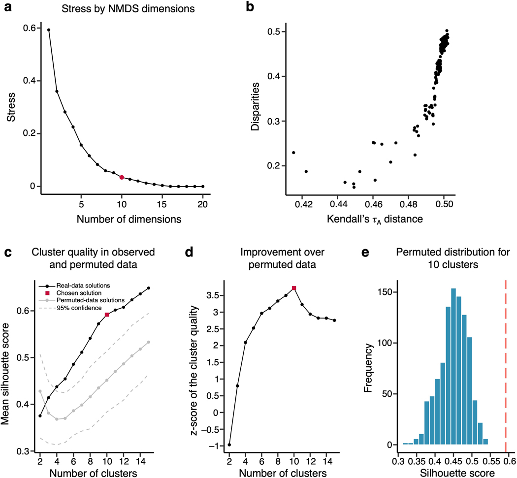
To cluster pain-predictive brain regions based on the patterns of the representational distance across individuals, we first vectorized the normalized RDMs acquired in the multivariate analysis of the discovery dataset and used them as inputs for the representational connectivity analysis²³. By calculating Kendall’s τ_A among the brain regions, we obtained a 21 × 21 representational connectivity matrix, which was used as the basis for the region clustering. For clustering, we transformed the Kendall’s τ_A matrix into a distance matrix by calculating (1 – Kendall’s τ_A )/2, where values ranged from 0 to 1, with 0 indicating identity and 1 indicating the maximum distance. Then, we applied the nonmetric multidimensional scaling (NMDS) to the Kendall’s τ_A distance matrix. To select the appropriate number of NMDS dimensions, we evaluated the stress metric of the NMDS solutions ranging from 1 to 20 dimensions and selected the final number of dimensions, which was 10, based on the scree test (Extended Data Fig. 8a). Finally, we performed hierarchical clustering with average linkage on the selected NMDS results and used permutation tests to choose the number of clusters k. In particular, for each possible solution ranging from 2 to 15 clusters, we first evaluated the mean clustering quality q in the observed data using the silhouette values computed as

$$q=\frac{1}{i}\sum _i\frac{d_{i_{nn}}-d_{i_w}}{\mathrm{m}\mathrm{a}\mathrm{x}(d_{ic},d_{inn})}$$

where i denotes the region number, $d_{i_{nn}}$ is the distance from a region to the nearest neighboring cluster, and $d_{i_w}$ is the Euclidean distance from a region to the center of its own cluster. Then, we permuted the NMDS scores, applied the same clustering algorithm, and evaluated q of the clustering solutions based on the permuted data. We ran 1,000 iterations of the process to create a null-hypothesis distribution for the clustering quality q, which allowed us to assess the z-scores for q of each clustering solution of the observed data as follows

$$Z_k=\frac{q_{obs}-{\stackrel{-}{q}}_{null}}{\sqrt{\frac{\sum _1^N{\left(q_{null}-{\stackrel{-}{q}}_{null}\right)}^2}{N-1}}}$$

where k denotes the cluster number, $q_{obs}$ is the clustering quality of the original data, $q_{null}$ is the clustering quality of the permuted data, and N is the number of iterations (Extended Data Fig. 8d). See refs. ^66,67 for other example use of the analysis.

Principal gradient analysis

To examine where our region clusters were on the spectrum of the principal gradient of the cortical organization that ranges from unimodal to transmodal areas, as suggested by a previous study²⁴, we calculated the mean principal gradient in the clusters. We first masked a principal gradient map derived from an independent resting-state fMRI dataset (N = 59) with the region clusters. Then, we calculated the mean value in each cluster. For comparison with the mean residualized representational distance, we assigned ranks to the region clusters based on the principal gradient values and mean representational distance and calculated the rank correlation between them.

Statistics and reproducibility

The analyses were performed on 14 studies including 11 published studies. The total sample size was N = 528, which was much larger than sample sizes common in experimental fMRI studies⁶⁸. For this reason, we did not conduct formal statistical tests to predetermine the sample size. In one study (Study 8), 4 participants were excluded due to the unsuccessful extraction of the single-trial data. In all studies, the stimuli were fully randomized within subjects. Data collection and analysis were not performed blind to the conditions of the experiments.

In Fig. 1b, the top 10% of the mean negative logarithmic p-values across all 404 individualized maps are displayed. To obtain the p-values, we first ran bootstrap tests on each of the 404 individualized maps (with 10,000 samples), and then calculated the two-tailed uncorrected p-values from z-scores based on the distribution of weights resulting from the bootstrap tests. In Figs. 3b and 3d, we used Pearson’s correlation coefficient r with a subsequent t-test to determine two-tailed p values (n = 21 regions). In both Figs. 3c and 4a, we show the mean residualized representational distances and their standard errors of the mean. The standard error of the mean was calculated across all pair comparisons of individuals, i.e., C(404, 2) = 81,406. In Fig. 4b, c, we used Spearman’s rank correlation coefficient ρ with a subsequent t-test to determine two-tailed p-values. In Extended Data Fig. 3, to select individualized models with significant prediction performance, we evaluated Pearson’s correlation coefficient between the predicted and actual outcome values and conducted t-test with the correction for multiple comparisons using False Discovery Rate at q < 0.05. In Extended Data Figs. 3c (n = 21), 5c-e (n = 21), and 9c (n = 10), we used Spearman’s rank correlation coefficient ρ with a subsequent t-test to determine two-tailed p-values. The mean and standard error of the mean are shown in Extended Data Fig. 3a (based on all pair comparisons of n = 248), Extended Data Fig. 5a, b(based on all pair comparisons of n = 229 and n = 175, respectively), Extended Data Fig. 6c, d(based on all pair comparisons of n = 285 in both), and Extended Data Fig. 9d (based on all pair comparisons of n = 124). In Extended Data Fig. 8c, we show the mean and 95% confidence interval for clustering quality obtained from a permutation test of 1,000 samples. In Extended Data Fig. 8d, we calculated the z-scores for the clustering quality based on the permutation test and the observed clustering quality. Further details on the statistical analyses are reported in the relevant sections.

Reporting Summary

Further information on research design is available in the Nature Research Reporting Summary linked to this article.

Data Availability

The individualized pain-predictive maps from the discovery dataset, region masks and regional normalized representational dissimilarity matrices are available at https://github.com/cocoanlab/individual_var_pain. The cerebral and cerebellar atlases used in this study are available at https://github.com/canlab/CanlabCore/tree/master/CanlabCore/canlab_canonical_brains/Combined_multiatlas_ROI_masks. The data from the replication dataset are available upon request.

Code Availability

In-house Matlab codes for fMRI data analyses used in this study are available at https://github.com/canlab/CanlabCore. An example code for the multivariate representational similarity analysis is available at https://github.com/cocoanlab/individual_var_pain.

Extended Data

Extended Data Fig. 1. Reference results based on pain signatures and large-scale functional networks.

To provide a reference to other commonly used brain parcellations and existing pain signatures, we performed the analyses presented in the manuscript with the NPS¹, SIIPS1² (thresholded at q < 0.05, false discovery rate [FDR] correction), and seven large-scale resting-state functional networks³ as masks. (a) The plot shows the proportions of the overlapping voxels of the pain signature and network masks with the area of the important voxels identified in the current study. (b) and (c) show the voxel-wise variance across the individuals from the discovery dataset in the thresholded NPS and SIIPS1 masks, respectively. (d) In each signature and network mask, we calculated the mean importance with mean(-log(p)) (based on two-tailed p-values) and the mean voxel-wise variance. The results suggest that the limbic network showed the highest mean variance, while the dorsal attention network showed the lowest mean variance (e) We also performed the multivariate analysis. we calculated the inter-individual representational dissimilarity matrix (RDM) using the correlation-based distance for each masked area, performed the permutation tests with 1,000 samples, as we did in the main analyses, and calculated the normalized RDMs (z-scores), as we did in the main analysis (see Fig. 3a in the main manuscript). The results suggest that the limbic and visual networks showed the highest mean normalized representational distance (i.e., highest inter-individual variability), while the somatomotor and ventral attention networks showed the lowest distance (i.e., lower inter-individual variability). dAttention, dorsal attention network; vAttention, ventral attention network

Extended Data Fig. 2. Proportions of the signs of median predictive weights.

(a) We found the median weight across voxels for each participant in each region and calculated the proportion of positive and negative median weights across all subjects. The pie charts display the percentage of median positive weights in red and negative weights in blue. (b) The bar plot shows the ratio of the number of positive to the number of negative median weights in each region. The red bars depict the regions with more positive median weights, and the blue bars mark the regions with more negative median weights.

Extended Data Fig. 3. Results after removing predictive maps with non-significant prediction performance.

To examine the effects of individuals with poor prediction performance on the inter-individual variability, we conducted the same analyses only with the individualized models with significant performance after correction for multiple comparisons using FDR correction at q < 0.05. All analyses shown here were performed on a reduced dataset of n = 248 after removing n = 156 with non-significant prediction performance. (a) The plot shows the mean representational distance after regressing out the effects of the region size. The error bar indicates the standard error of the mean. This corresponds to Fig. 3c of the main manuscript, which used the whole discovery dataset. (b) The scatter plot depicts the univariate analysis result, that is, the mean voxel weight and variance in each region. This corresponds to Fig. 2c of the main manuscript. (c) We assigned ranks to each region based on the residualized representational distance in both the original result based on the whole dataset and in the result based on the reduced dataset presented here. The two sets of results were significantly correlated at Spearman’s ρ = 0.96, p = 0.00001, two-tailed.

Extended Data Fig. 4. Inspection of potential study-specific effects on results.

To evaluate any potential study-specific effects on our results, we compared the final results (both univariate and multivariate) with the results with one study removed. For the comparisons, we calculated Spearman’s $\rho$ using the rank orders of the brain regions’ individual variability between the results from the full versus reduced datasets. The blue dots show the results of the univariate analysis, ranging from 0.86 to 0.98, while the orange triangles are the results of the multivariate analysis, ranging from 0.98 to 0.99. The straight lines mark the mean Spearman’s $\rho$ for both cases with respective colors.

Extended Data Fig. 5. Results of the representational similarity analysis for studies with and without context manipulation.

We performed the representational similarity analysis and controlled for the region size in the discovery dataset divided into studies (a) with context manipulation (e.g., placebo and cognitive regulation; studies 1, 4, 6, 7, 8, 11, and 12; n = 229) and (b) without context manipulation (studies 2, 3, 5, 9, 10, and 13; n = 175). The figures show the mean residualized representational distance and the standard error of the mean. (c) We found a significant correlation between region ranks in (a) and (b) of Spearman’s ρ = 0.61, p = 0.004, two-tailed. When compared with the region ranks in the discovery set, both (d) result in studies with context manipulation and (e) result in studies without context manipulation showed significant correlations of ρ = 0.92, p = 4.2 × 10⁻⁶, and ρ = 0.83, p = 4.3 × 10⁻⁷, respectively, all two-tailed.

Extended Data Fig. 6. Results after excluding the studies that showed low prediction performance.

(a) The plot shows the average prediction performance of the individualized whole-brain SVR models across 13 studies. Studies 7, 12 and 13 (marked in red) had the lowest performance, mean r = 0.20, 0.19, and 0.04, respectively. To test whether these studies with low performance affected the results, we re-did the analysis without these studies, i.e., on n = 285 individuals. (b) The scatter plot shows the mean predictive weight and variance across the individualized maps for each region after the exclusion of the three studies. (c) The plot displays the mean representational distance (z-scores) and standard error of the mean in each region based on all pair comparisons of individuals, i.e., C(285, 2) = 40,470. (d) The residuals of the representational distance after removing the effects of the region size and the standard error of the mean based on all pair comparisons of individuals, i.e., C(285, 2) = 40,470, are plotted.

Extended Data Fig. 7. tSNR map.

The group average of tSNR is visualized on a brain underlay with brighter colors depicting higher tSNR values, i.e., better tSNR.

Extended Data Fig. 8. Nonmetric multidimensional scaling-based hierarchical clustering analysis.

(a) For the clustering of pain-predictive regions, we first ran the nonmetric multidimensional scaling (NMDS) on the Kendall’s τ_A distance matrix, which was calculated as (1 – Kendall’s τ_A)/2. Based on the stress metric and scree method, we selected 10 dimensions (marked in red). (b) The x-axis of the scatter plot shows the input Kendall’s τ_A distance between regions, and the y-axis shows the Euclidean distance between the regions scaled into 10 dimensions after the NMDS. (c) We performed the hierarchical clustering with average linkage on the selected NMDS results and used permutation tests to choose the final number of clusters, k. For the permutation tests, we shuffled the NMDS scores, applied the clustering algorithm, and assessed the clustering quality of the permuted data at each iteration. We ran a total of 1,000 iterations, and the plot shows the mean cluster quality of both the observed (solid black line) and permuted (solid gray line) data, as well as the 95% confidence interval (gray dashed lines) for the permuted cluster quality. The red square marks the selected solution with a Silhouette score of 0.59. (d) The plot shows the z-scores that indicate an improvement of the cluster quality of the observed data compared to the permuted null data. The highest improvement was achieved with the 10 cluster solution (shown as the red square) with a z-score of 3.72, p = 0.0002, two-tailed. (e) The histogram depicts the observed cluster quality of the 10 cluster solution (red dashed line) versus the null distribution from the permutation test (blue histogram).

Extended Data Fig. 9. Cross-individual pain prediction.

To further illustrate the inter-individual variability in pain representations across different region clusters, we conducted cross-individual prediction of pain using pain predictive patterns of region clusters in Study 14. The panels (a) and (b) show examples of the cross-prediction using the vmPFC (the most variable region cluster) and a/pMCC/SMA/SMC (the most stable region cluster) cluster patterns, respectively. The gray lines in the line plots show the mean regression lines of pain prediction in others using an individual’s predictive map (i.e., each line indicates the prediction using one participant’s pain prediction model). The black lines show the global average of all the individual regression lines. The violin plots show the mean correlation between the predicted and actual pain ratings in cross-individual pain prediction. Each dot represents mean prediction-outcome correlation using one participant’s pain prediction model. (c) We calculated the global cross-individual prediction performance of each region cluster using prediction-outcome correlations. The top panel shows the relationship between the rank in the mean residualized distance (y-axis), where clusters are ordered from the most variable to the least variable cluster, and the rank in the correlation values (x-axis), where the clusters are ordered from the lowest to the highest cross-individual prediction performance. Together with the examples in (a) and (b), this plot suggests that the cross-individual prediction is more reliable in the clusters with lower inter-individual variability. (d) The plot displays the mean correlation values with the standard error of the mean for each region cluster based on n = 124.

Extended Data Fig. 10. Relationship between the principal gradient of functional connectivity and mean residualized representational distance.

To compare the principal gradient spectrum and mean residualized distance in clusters, we first calculated the principal gradient map using our own resting-state fMRI dataset (n = 56; 7-min resting scan) to create a volumetric principal gradient image and to include the subcortical regions. We assigned ranks to the region clusters based on both the principal gradient value (x-axis) and mean residualized distance (y-axis) and compared them using Spearman’s rank correlation coefficient. We found a significant relationship at Spearman’s ρ = 0.68, p = 0.04, two-tailed.

References

- 1.Coghill RC The Distributed Nociceptive System: A Framework for Understanding Pain. Trends Neurosci, doi: 10.1016/j.tins.2020.07.004 (2020). [DOI] [PMC free article] [PubMed] [Google Scholar]
- 2.Tracey I. & Mantyh PW The cerebral signature for pain perception and its modulation. Neuron 55, 377–391, doi: 10.1016/j.neuron.2007.07.012 (2007). [DOI] [PubMed] [Google Scholar]
- 3.Apkarian AV, Bushnell MC, Treede RD & Zubieta JK Human brain mechanisms of pain perception and regulation in health and disease. Eur J Pain 9, 463–484, doi: 10.1016/j.ejpain.2004.11.001 (2005). [DOI] [PubMed] [Google Scholar]
- 4.Xu A. et al. Convergent neural representations of experimentally-induced acute pain in healthy volunteers: A large-scale fMRI meta-analysis. Neurosci Biobehav Rev 112, 300–323, doi: 10.1016/j.neubiorev.2020.01.004 (2020). [DOI] [PMC free article] [PubMed] [Google Scholar]
- 5.Kucyi A. & Davis KD The dynamic pain connectome. Trends Neurosci 38, 86–95, doi: 10.1016/j.tins.2014.11.006 (2015). [DOI] [PubMed] [Google Scholar]
- 6.Greenspan JD, Lee RR & Lenz FA Pain sensitivity alterations as a function of lesion location in the parasylvian cortex. Pain 81, 273–282, doi:Doi 10.1016/S0304-3959(99)00021-4 (1999). [DOI] [PubMed] [Google Scholar]
- 7.Greenspan JD et al. Quantitative somatic sensory testing and functional imaging of the response to painful stimuli before and after cingulotomy for obsessive-compulsive disorder (OCD). Eur J Pain 12, 990–999, doi: 10.1016/j.ejpain.2008.01.007 (2008). [DOI] [PMC free article] [PubMed] [Google Scholar]
- 8.Valet M. et al. Distraction modulates connectivity of the cingulo-frontal cortex and the midbrain during pain--an fMRI analysis. Pain 109, 399–408, doi: 10.1016/j.pain.2004.02.033 (2004). [DOI] [PubMed] [Google Scholar]
- 9.Berna C. et al. Induction of Depressed Mood Disrupts Emotion Regulation Neurocircuitry and Enhances Pain Unpleasantness. Biological Psychiatry 67, 1083–1090, doi: 10.1016/j.biopsych.2010.01.014 (2010). [DOI] [PubMed] [Google Scholar]
- 10.López-Solà M, Koban L. & Wager TD Transforming pain with prosocial meaning: an fMRI study. Psychosomatic medicine 80, 814 (2018). [DOI] [PMC free article] [PubMed] [Google Scholar]
- 11.Losin EAR et al. Neural and sociocultural mediators of ethnic differences in pain. Nat Hum Behav, doi: 10.1038/s41562-020-0819-8 (2020). [DOI] [PMC free article] [PubMed] [Google Scholar]
- 12.Hashmi JA & Davis KD Deconstructing sex differences in pain sensitivity. Pain 155, 10–13, doi: 10.1016/j.pain.2013.07.039 (2014). [DOI] [PubMed] [Google Scholar]
- 13.Raja SN et al. The revised International Association for the Study of Pain definition of pain: concepts, challenges, and compromises. Pain (2020). [DOI] [PMC free article] [PubMed] [Google Scholar]
- 14.Gordon EM et al. Precision Functional Mapping of Individual Human Brains. Neuron 95, 791–807, doi: 10.1016/j.neuron.2017.07.011 (2017). [DOI] [PMC free article] [PubMed] [Google Scholar]
- 15.Laumann TO et al. Functional System and Areal Organization of a Highly Sampled Individual Human Brain. Neuron 87, 657–670, doi: 10.1016/j.neuron.2015.06.037 (2015). [DOI] [PMC free article] [PubMed] [Google Scholar]
- 16.Davis KD et al. Discovery and validation of biomarkers to aid the development of safe and effective pain therapeutics: challenges and opportunities. Nat Rev Neurol 16, 381–400, doi: 10.1038/s41582-020-0362-2 (2020). [DOI] [PMC free article] [PubMed] [Google Scholar]
- 17.Wager TD et al. An fMRI-Based Neurologic Signature of Physical Pain. New Engl J Med 368, 1388–1397, doi: 10.1056/NEJMoa1204471 (2013). [DOI] [PMC free article] [PubMed] [Google Scholar]
- 18.Lee JJ et al. A neuroimaging biomarker for sustained experimental and clinical pain. Nat Med 27, 174–182, doi: 10.1038/s41591-020-1142-7 (2021). [DOI] [PMC free article] [PubMed] [Google Scholar]
- 19.Woo C-W et al. Quantifying cerebral contributions to pain beyond nociception. Nat Commun 8 (2017). [DOI] [PMC free article] [PubMed] [Google Scholar]
- 20.Yeo BT et al. The organization of the human cerebral cortex estimated by intrinsic functional connectivity. J Neurophysiol 106, 1125–1165, doi: 10.1152/jn.00338.2011 (2011). [DOI] [PMC free article] [PubMed] [Google Scholar]
- 21.Kragel PA, Koban L, Barrett LF & Wager TD Representation, Pattern Information, and Brain Signatures: From Neurons to Neuroimaging. Neuron 99, 257–273, doi: 10.1016/j.neuron.2018.06.009 (2018). [DOI] [PMC free article] [PubMed] [Google Scholar]
- 22.Hong YW, Yoo Y, Han J, Wager TD & Woo CW False-positive neuroimaging: Undisclosed flexibility in testing spatial hypotheses allows presenting anything as a replicated finding. Neuroimage 195, 384–395, doi: 10.1016/j.neuroimage.2019.03.070 (2019). [DOI] [PubMed] [Google Scholar]
- 23.Kriegeskorte N, Mur M. & Bandettini P. Representational similarity analysis–connecting the branches of systems neuroscience. Frontiers in systems neuroscience 2 (2008). [DOI] [PMC free article] [PubMed] [Google Scholar]
- 24.Margulies DS et al. Situating the default-mode network along a principal gradient of macroscale cortical organization. Proc Natl Acad Sci U S A 113, 12574–12579, doi: 10.1073/pnas.1608282113 (2016). [DOI] [PMC free article] [PubMed] [Google Scholar]
- 25.Favilla S. et al. Ranking brain areas encoding the perceived level of pain from fMRI data. Neuroimage 90, 153–162, doi: 10.1016/j.neuroimage.2014.01.001 (2014). [DOI] [PubMed] [Google Scholar]
- 26.Kong J. et al. Exploring the brain in pain: activations, deactivations and their relation. Pain 148, 257–267, doi: 10.1016/j.pain.2009.11.008 (2010). [DOI] [PMC free article] [PubMed] [Google Scholar]
- 27.Senkowski D, Hofle M. & Engel AK Crossmodal shaping of pain: a multisensory approach to nociception. Trends in Cognitive Sciences 18, 319–327, doi: 10.1016/j.tics.2014.03.005 (2014). [DOI] [PubMed] [Google Scholar]
- 28.Elkhetali AS, Vaden RJ, Pool SM & Visscher KM Early visual cortex reflects initiation and maintenance of task set. Neuroimage 107, 277–288 (2015). [DOI] [PMC free article] [PubMed] [Google Scholar]
- 29.Seminowicz DA & Davis KD Interactions of pain intensity and cognitive load: the brain stays on task. Cereb Cortex 17, 1412–1422 (2007). [DOI] [PubMed] [Google Scholar]
- 30.Dum RP, Levinthal DJ & Strick PL The spinothalamic system targets motor and sensory areas in the cerebral cortex of monkeys. J Neurosci 29, 14223–14235, doi: 10.1523/JNEUROSCI.3398-09.2009 (2009). [DOI] [PMC free article] [PubMed] [Google Scholar]
- 31.Almeida TF, Roizenblatt S. & Tufik S. Afferent pain pathways: a neuroanatomical review. Brain research 1000, 40–56 (2004). [DOI] [PubMed] [Google Scholar]
- 32.Shackman AJ et al. The integration of negative affect, pain and cognitive control in the cingulate cortex. Nat Rev Neurosci 12, 154–167, doi: 10.1038/nrn2994 (2011). [DOI] [PMC free article] [PubMed] [Google Scholar]
- 33.Tan LL et al. A pathway from midcingulate cortex to posterior insula gates nociceptive hypersensitivity. Nat Neurosci 20, 1591–1601, doi: 10.1038/nn.4645 (2017). [DOI] [PubMed] [Google Scholar]
- 34.Kulkarni B. et al. Attention to pain localization and unpleasantness discriminates the functions of the medial and lateral pain systems. Eur J Neurosci 21, 3133–3142, doi: 10.1111/j.1460-9568.2005.04098.x (2005). [DOI] [PubMed] [Google Scholar]
- 35.Hutchison WD, Davis KD, Lozano AM, Tasker RR & Dostrovsky JO Pain-related neurons in the human cingulate cortex. Nat Neurosci 2, 403–405, doi: 10.1038/8065 (1999). [DOI] [PubMed] [Google Scholar]
- 36.Kragel PA et al. Generalizable representations of pain, cognitive control, and negative emotion in medial frontal cortex. Nature Neuroscience 21, 283-+, doi: 10.1038/s41593-017-0051-7 (2018). [DOI] [PMC free article] [PubMed] [Google Scholar]
- 37.Segerdahl AR, Mezue M, Okell TW, Farrar JT & Tracey I. The dorsal posterior insula subserves a fundamental role in human pain. Nat Neurosci 18, 499–500, doi: 10.1038/nn.3969 (2015). [DOI] [PMC free article] [PubMed] [Google Scholar]
- 38.Kross E, Berman MG, Mischel W, Smith EE & Wager TD Social rejection shares somatosensory representations with physical pain. Proceedings of the National Academy of Sciences 108, 6270–6275 (2011). [DOI] [PMC free article] [PubMed] [Google Scholar]
- 39.Evrard HC, Logothetis NK & Craig AD Modular architectonic organization of the insula in the macaque monkey. J Comp Neurol 522, 64–97, doi: 10.1002/cne.23436 (2014). [DOI] [PubMed] [Google Scholar]
- 40.Ashar YK, Chang LJ & Wager TD Brain mechanisms of the placebo effect: an affective appraisal account. Annual review of clinical psychology 13, 73–98 (2017). [DOI] [PubMed] [Google Scholar]
- 41.Woo C-W, Roy M, Buhle JT & Wager TD Distinct brain systems mediate the effects of nociceptive input and self-regulation on pain. Plos Biol 13, e1002036 (2015). [DOI] [PMC free article] [PubMed] [Google Scholar]
- 42.Seminowicz DA & Davis KD Cortical responses to pain in healthy individuals depends on pain catastrophizing. Pain 120, 297–306, doi: 10.1016/j.pain.2005.11.008 (2006). [DOI] [PubMed] [Google Scholar]
- 43.Tinnermann A, Geuter S, Sprenger C, Finsterbusch J. & Buchel C. Interactions between brain and spinal cord mediate value effects in nocebo hyperalgesia. Science 358, 105–108, doi: 10.1126/science.aan1221 (2017). [DOI] [PubMed] [Google Scholar]
- 44.Bonnici HM & Maguire EA Two years later–Revisiting autobiographical memory representations in vmPFC and hippocampus. Neuropsychologia 110, 159–169 (2018). [DOI] [PMC free article] [PubMed] [Google Scholar]
- 45.Ciaramelli E, De Luca F, Monk AM, McCormick C. & Maguire EA What” wins” in VMPFC: Scenes, situations, or schema? Neuroscience & Biobehavioral Reviews (2019). [DOI] [PubMed] [Google Scholar]
- 46.Zunhammer M, Spisak T, Wager TD, Bingel U. & Placebo Imaging C. Meta-analysis of neural systems underlying placebo analgesia from individual participant fMRI data. Nat Commun 12, 1391, doi: 10.1038/s41467-021-21179-3 (2021). [DOI] [PMC free article] [PubMed] [Google Scholar]
- 47.Claassen J. et al. Cerebellum is more concerned about visceral than somatic pain. Journal of Neurology, Neurosurgery & Psychiatry 91, 218–219 (2020). [DOI] [PubMed] [Google Scholar]
- 48.Huntenburg JM, Bazin PL & Margulies DS Large-Scale Gradients in Human Cortical Organization. Trends Cogn Sci 22, 21–31, doi: 10.1016/j.tics.2017.11.002 (2018). [DOI] [PubMed] [Google Scholar]
- 49.Finn ES et al. Functional connectome fingerprinting: identifying individuals using patterns of brain connectivity. Nature neuroscience 18, 1664 (2015). [DOI] [PMC free article] [PubMed] [Google Scholar]
- 50.Farrell SM, Green A. & Aziz T. The Current State of Deep Brain Stimulation for Chronic Pain and Its Context in Other Forms of Neuromodulation. Brain Sci 8, doi: 10.3390/brainsci8080158 (2018). [DOI] [PMC free article] [PubMed] [Google Scholar]
- 51.Yang S. & Chang MC Effect of Repetitive Transcranial Magnetic Stimulation on Pain Management: A Systematic Narrative Review. Front Neurol 11, 114, doi: 10.3389/fneur.2020.00114 (2020). [DOI] [PMC free article] [PubMed] [Google Scholar]
- 52.Zhang S. et al. Pain Control by Co-adaptive Learning in a Brain-Machine Interface. Curr Biol 30, 3935–3944 e3937, doi: 10.1016/j.cub.2020.07.066 (2020). [DOI] [PMC free article] [PubMed] [Google Scholar]
- 53.Meloto CB et al. Human pain genetics database: a resource dedicated to human pain genetics research. Pain 159, 749–763, doi: 10.1097/j.pain.0000000000001135 (2018). [DOI] [PubMed] [Google Scholar]
- 54.Kohl A, Rief W. & Glombiewski JA Acceptance, Cognitive Restructuring, and Distraction as Coping Strategies for Acute Pain. Journal of Pain 14, 305–315, doi: 10.1016/j.jpain.2012.12.005 (2013). [DOI] [PubMed] [Google Scholar]
- 55.Coghill RC, McHaffie JG & Yen YF Neural correlates of interindividual differences in the subjective experience of pain. Proc Natl Acad Sci U S A 100, 8538–8542, doi: 10.1073/pnas.1430684100 (2003). [DOI] [PMC free article] [PubMed] [Google Scholar]
- 56.Mehta S. et al. Identification and Characterization of Unique Subgroups of Chronic Pain Individuals with Dispositional Personality Traits. Pain Res Manag 2016, doi: 10.1155/2016/5187631 (2016). [DOI] [PMC free article] [PubMed] [Google Scholar]
- 57.Haxby JV et al. A common, high-dimensional model of the representational space in human ventral temporal cortex. Neuron 72, 404–416, doi: 10.1016/j.neuron.2011.08.026 (2011). [DOI] [PMC free article] [PubMed] [Google Scholar]
- 58.Coghill RC, Gilron I. & Iadarola MJ Hemispheric lateralization of somatosensory processing. J Neurophysiol 85, 2602–2612, doi: 10.1152/jn.2001.85.6.2602 (2001). [DOI] [PubMed] [Google Scholar]
- 59.Pruim RHR et al. ICA-AROMA: A robust ICA-based strategy for removing motion artifacts from fMRI data. Neuroimage 112, 267–277, doi: 10.1016/j.neuroimage.2015.02.064 (2015). [DOI] [PubMed] [Google Scholar]
- 60.Atlas LY, Bolger N, Lindquist MA & Wager TD Brain mediators of predictive cue effects on perceived pain. J Neurosci 30, 12964–12977, doi: 10.1523/JNEUROSCI.0057-10.2010 (2010). [DOI] [PMC free article] [PubMed] [Google Scholar]
- 61.Atlas LY, Lindquist MA, Bolger N. & Wager TD Brain mediators of the effects of noxious heat on pain. Pain 155, 1632–1648, doi: 10.1016/j.pain.2014.05.015 (2014). [DOI] [PMC free article] [PubMed] [Google Scholar]
- 62.Wager TD & Nichols TE Optimization of experimental design in fMRI: a general framework using a genetic algorithm. Neuroimage 18, 293–309, doi: 10.1016/S1053-8119(02)00046–0 (2003). [DOI] [PubMed] [Google Scholar]
- 63.Lindquist MA & Gelman A. Correlations and Multiple Comparisons in Functional Imaging: A Statistical Perspective (Commentary on Vul et al., 2009). Perspect Psychol Sci 4, 310–313, doi: 10.1111/j.1745-6924.2009.01130.x (2009). [DOI] [PubMed] [Google Scholar]
- 64.Diedrichsen J, Balsters JH, Flavell J, Cussans E. & Ramnani N. A probabilistic MR atlas of the human cerebellum. Neuroimage 46, 39–46, doi: 10.1016/j.neuroimage.2009.01.045 (2009). [DOI] [PubMed] [Google Scholar]
- 65.Shattuck DW et al. Construction of a 3D probabilistic atlas of human cortical structures. Neuroimage 39, 1064–1080, doi: 10.1016/j.neuroimage.2007.09.031 (2008). [DOI] [PMC free article] [PubMed] [Google Scholar]
- 66.Wager TD, Scott DJ & Zubieta JK Placebo effects on human mu-opioid activity during pain. Proc Natl Acad Sci U S A 104, 11056–11061, doi: 10.1073/pnas.0702413104 (2007). [DOI] [PMC free article] [PubMed] [Google Scholar]
- 67.Wager TD, Davidson ML, Hughes BL, Lindquist MA & Ochsner KN Prefrontal-subcortical pathways mediating successful emotion regulation. Neuron 59, 1037–1050, doi: 10.1016/j.neuron.2008.09.006 (2008). [DOI] [PMC free article] [PubMed] [Google Scholar]
- 68.Szucs D. & Ioannidis JP Sample size evolution in neuroimaging research: An evaluation of highly-cited studies (1990–2012) and of latest practices (2017–2018) in high-impact journals. Neuroimage 221, 117164, doi: 10.1016/j.neuroimage.2020.117164 (2020). [DOI] [PubMed] [Google Scholar]
Associated Data
This section collects any data citations, data availability statements, or supplementary materials included in this article.
Supplementary Materials
Data Availability Statement