The role of the airline transportation network in the prediction and predictability of global epidemics

Abstract

The systematic study of large-scale networks has unveiled the ubiquitous presence of connectivity patterns characterized by large-scale heterogeneities and unbounded statistical fluctuations. These features affect dramatically the behavior of the diffusion processes occurring on networks, determining the ensuing statistical properties of their evolution pattern and dynamics. In this article, we present a stochastic computational framework for the forecast of global epidemics that considers the complete worldwide air travel infrastructure complemented with census population data. We address two basic issues in global epidemic modeling: (i) we study the role of the large scale properties of the airline transportation network in determining the global diffusion pattern of emerging diseases; and (ii) we evaluate the reliability of forecasts and outbreak scenarios with respect to the intrinsic stochasticity of disease transmission and traffic flows. To address these issues we define a set of quantitative measures able to characterize the level of heterogeneity and predictability of the epidemic pattern. These measures may be used for the analysis of containment policies and epidemic risk assessment.

The mathematical modeling of epidemics has often dealt with the predictions and predictability of outbreaks in real populations with complicated social and spatial structures and with heterogeneous patterns in the contact network (1–8). All these factors have led to sophisticate modeling approaches including disease realism, metapopulation grouping, and stochasticity, and more recently to agent-based numerical simulations that recreate entire populations and their dynamics at the scale of the single individual (9, 10). In many instances, however, the introduction of the inherent complex features and emerging properties (11–13) of the network in which epidemics occur implies the breakdown of standard homogeneous approaches (5, 6) and calls for a systematic investigation of the impact of the detailed system’s characteristics in the evolution of the epidemic outbreak. These considerations are particularly relevant in the study of the geographical spread of epidemics where the various long-range heterogeneous connections typical of modern transportation networks naturally give rise to a very complicated evolution of epidemics characterized by heterogeneous and seemingly erratic outbreaks (14, 15), as recently documented in the severe acute respiratory syndrome case (www.who.int/csr/sars/en). In this context, air-transportation represents a major channel of epidemic propagation, as pointed out in the modeling approach to global epidemic diffusion of Rvachev and Longini (16) capitalizing on previous studies on the Russian airline network (17). Similar modeling approaches, even if limited by a partial knowledge of the worldwide transportation network, have been used to study specific outbreaks such as pandemic influenza (18–20), HIV (21), and, very recently, severe acute respiratory syndrome (22). The availability of the complete worldwide airport network (WAN) data set and the recent extensive studies of its topology (23, 24) are finally allowing a full-scale computational study of global epidemics. In the following article, we will consider a global stochastic epidemic model including the full International Air Transport Association (www.iata.org) database, aiming at a detailed study of the interplay among the network structure and the stochastic features of the infection dynamics in defining the global spreading of epidemics. In particular, whereas previous studies have generally been focused in the a posteriori analysis of real case studies of global epidemics, the large-scale modeling presented here allows us to address more basic theoretical issues such as the statistical properties of the epidemic pattern and the effect on it of the complex architecture of the underlying transportation network. Finally, such a detailed level of description allows for the quantitative assessment of the reliability of the obtained forecast with respect to the stochastic nature of the disease transmission and travel flows, the outbreak initial conditions, and the network structure.

Results and Discussion

The Air-Transportation-Network Heterogeneity.

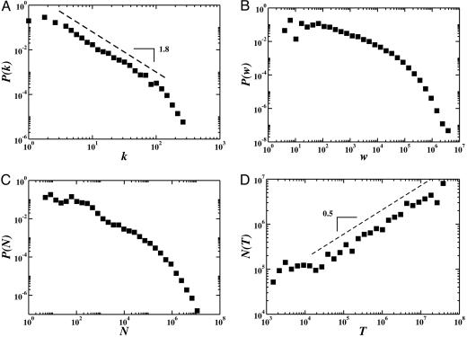
The International Air Transport Association database contains the world list of airport pairs connected by direct flights and the number of available seats on any given connection for the year 2002. The resulting worldwide air-transportation network (WAN) is therefore a weighted graph comprising V = 3,880 vertices denoting airports and E = 18,810 weighted edges whose weight w_jl accounts for the passenger flow between the airports j and l. This data set has been complemented by the population N_j of the large metropolitan area served by the airport as obtained by different sources. The final network data set contains the 3,100 largest airports, 17,182 edges (accounting for 99% of the worldwide traffic), and the respective urban population data. The obtained network is highly heterogeneous both in the connectivity pattern and the traffic capacities (see Fig. 1). The probability distributions that an airport j has k_j connections (degree) to other airports and handles a number T_j = Σ_lw_jl of passengers (traffic) exhibit heavy-tails and very large statistical fluctuations (23, 24). Analogously, the probability that a connection has a traffic w is skewed and heavy-tailed. Finally, the city population N is heavy-tailed distributed in agreement with the general result of Zipf’s law for the city size (25). More strikingly, these quantities appear to have nonlinear associations among them. This is clearly shown by the behavior relating the traffic handled by each airport T with the corresponding number of connections k that follows the nonlinear form T ≈ k^β with β ≅ 1.5 (23). Analogously, the city population and the traffic handled by the corresponding airport follows the nonlinear relation N ≈ T^α with α ≅ 0.5 in contrast with the linear behavior assumed in a previous analysis (22). The presence of broad statistical distributions and nonlinear relations among the various quantities indicate a possible major impact in the ensuing disease spreading pattern.

Fig. 1.

Properties of the worldwide airport network. Statistical fluctuations are observed over a broad range of length scales. (A) The degree distribution P(k) follows a power-law behavior on almost two decades with exponent 18 ± 0.2. (B) The distribution of the weights (fluxes) is skewed and heavy-tailed. (C) The distribution of populations is heavy-tailed distributed, in agreement with the commonly observed Zipf’s law (25). (D) The city population varies with the traffic of the corresponding airport as N ≈ T^α with α ≅ 0.5, in contrast with the linear behavior postulated in previous works (22).

Modeling Global Epidemics.

As a basic element of our modeling approach we assume the basic standard compartmentalization in which each individual can only exist in one of the discrete states such as susceptible (S), latent (L), infected (I), permanently recovered (R), etc. In each city j, the population is N_j and X_j^[m](t) is the number of individuals in the state [m] at time t. By definition, it follows that N_j = Σ_mX_j^[m](t). In each city j, the individuals are allowed to travel from one city to another by means of the airline transportation network and to change compartment because of the infection dynamics in each city, similarly to the models in refs. 16, 19, and 21 and the stochastic generalization of ref. 22. The dynamics of individuals due to travels between cities is described by the stochastic transport operator Ω_j({X^[m]}) representing the net balance of individuals in a given state X^[m] that entered and left each city j. This operator is a function of the traffic flows with the neighboring cities w_jl per unit time and the city populations N_j (for its explicit expression, see Materials and Methods) and might also include transit passengers on connecting flights. In each city, the dynamics of the individuals X_j^[m] between the different compartments assumes a fully mixed population and depends on the specific disease studied. The homogeneous assumption allows for a description of the disease evolution in terms of differential equations. In the present approach, we go beyond the simple deterministic approximation and use epidemic stochastic differential equations (22) with noise terms derived from the Langevin formulation of the epidemic reaction rate equations (26–29). The stochastic epidemic equations are then coupled among them by the stochastic transport operator Ω_j({X^[m]}) that describes movements of individuals among cities. The epidemic evolution is therefore obtained by solving numerically this set of coupled differential equations as reported in Materials and Methods.

Susceptible–Infected–Removed (SIR) Dynamics.

Global epidemic forecast would be extremely relevant in the case of the emergence of a new pandemic influenza that in general spreads rapidly with substantial transmission occurring before the onset of case-defining symptoms. For this reason, as a specific disease dynamics, we use the very simplistic approximation of the SIR that can be considered as the minimal model for a pandemic spread. This model provides a general discussion that is not hindered by the use of very complicate disease transmission mechanisms. Specific characteristics such as latency, incubation, and seasonal effects of the disease can be, however, easily implemented in the present framework (16). The analysis of two case studies and the comparison of the forecasts obtained with the present approach and the real data will be presented elsewhere. In the SIR model, the population Nj of each city is given by N_j = S_j(t) + I_j(t) + R_j(t), where S_j, I_j, and R_j represent the number of susceptible, infected, and recovered individuals at time t, respectively. The epidemic evolution is governed by the basic dynamical evolution of the SIR model where the probability that a susceptible individual acquires the infection from any given infected individual in the time interval dt is proportional to βdt, where β is the transmission parameter that captures the aetiology of the infection process. At the same time, infected individuals recover with a probability μdt, where μ⁻¹ is the average duration of the infection. Following the procedure outlined in Materials and Methods, we obtain the corresponding set of coupled differential equations (in this case three for each city) whose numerical integration provides the disease evolution in the 3,100 city considered. In the following, the results shown refer to this specific disease dynamics.

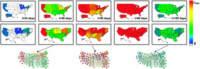
At first instance, it is possible to monitor standard epidemiological quantities such as the level of infected individuals, the morbidity, and the prevalence at different granularity levels; i.e., country, state, or administrative regions. In Fig. 2, we show the dynamical evolution in the United States of an epidemic starting in Hong Kong. The evolution of epidemic outbreaks is monitored by recording at each time step (1 day) the density of individuals in each state (S, I, and R) present in each city. The parameters β and μ are chosen according to ref. 20 in order to use biologically sound values and kept constant during the evolution (different values do not lead to different overall conclusions). This corresponds to assume that no restrictions on traveling or targeted prophylaxis measures are implemented during the outbreak. We group the states in the nine influenza surveillance regions that are identical to the nine divisions of the United States census and use two different visualization strategies. In the first set of maps, regions are drawn with their normal size, and a color code gives the prevalence of the infection in each region; i.e., the fraction of infected individuals. This representation readily shows the high heterogeneity of the pandemic evolution. Although useful, such visualization might be misleading because the same prevalence obtained in different regions might correspond to very different values in the number of infected individuals if the two regions are very differently populated. Moreover, it is common to find strong population-density heterogeneities, and it is not easy to detect visually a large level of contamination in a small but densely populated geographical area. To obtain a geographical representation that is able to carry at the same time information both on the level of infection and on the infection cases in each region, we have constructed the corresponding cartograms of the original maps in which the size of each geographic region (in our case United States influenza surveillance regions) is rescaled according to its population. Several methods for constructing cartograms have been developed (see ref. 30 and references therein), and here we have adopted the diffusion-based method (30), which produces cartograms by equalizing the population density through a linear diffusion process. The geographical map representation readily shows the heterogeneity of the spatiotemporal epidemic evolution, but a quantitative characterization of this heterogeneity and its relation with the air transportation network statistical properties are major issues that are not yet fully explored.

Fig. 2.

Geographical representation of the disease evolution in the United States for an epidemics starting in Hong Kong based on a SIR dynamics within each city. States are collected according to the nine influenza surveillance regions. The color code corresponds to the prevalence in each region, from 0to the maximum value reached (ρ_max). In the top row, the original United States maps are shown, and in the bottom are provided the corresponding cartograms obtained by rescaling each region according to its population. Three representations of the airport network restricted to the United States are also shown, in correspondence to the three different snapshots. The nodes represent the 100airports in the United States with highest traffic T; the color is assigned in accordance to the color code adopted for the maps.

Epidemic Heterogeneity and Network Structure.

To discriminate the role of the network structure on the spatiotemporal pattern of the epidemic process, we aim at a more quantitative analysis of its global heterogeneity. This heterogeneity might find its origin just in the stochastic nature of the infectious process or determined by the structural properties of the transportation network. In the latter case, it is possible to envision the possibility of a larger predictability of the epidemic behavior that would reflect the underlying network structure. Here, we introduce a characterization of the epidemic pattern by using the entropy, a quantity customarily used in information theory to quantify the level of disorder of a signal or system. At each time step, a snapshot of the epidemic pattern is provided by the set of values of the prevalence i_j(t) = I_j(t)/N_j in each city j. We can therefore define the normalized vector ρ⃗ with components ρ_j = i_j/Σ_li_l, which contains the relevant information on the epidemic pattern. In particular, we can measure the level of heterogeneity of the disease prevalence by measuring the disorder encoded in the vector ρ⃗ with the normalized entropy function H:

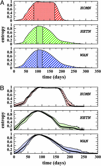
If the epidemics is homogeneously affecting all nodes (i.e., all prevalences are equal), the entropy attains its maximum value H = 1. Starting from H = 0, which corresponds to one initial infected city (the most localized and heterogeneous situation), H(t) increases as more cities become infected, thus reducing the level of heterogeneity (see Fig. 3A). It is important to stress that in the present context, the entropy does not have any thermodynamical meaning. It must be just considered as the appropriate mathematical tool able to quantify the statistical disorder of a complicate spatiotemporal signal.

Fig. 3.

Analysis of the heterogeneity of the epidemic pattern in the actual network (WAN) compared with the two network models (HOMN and HETN). A SIR dynamics is adopted within each city. (A) Entropy H(t) averaged over distinct initial infected cities and over noise realizations. Each profile is divided into three different phases, the central one corresponding to H > 0.9; i.e., to a homogeneous geographical spread of the disease. This phase is much longer for the HOMN than for the real airport network. The behavior observed in HETN is close to the real case meaning that the connectivity pattern plays a leading role in the epidemic behavior. (B) Average value of the entropy, with the maximal dispersion obtained from 2·10² noise realizations of an epidemics starting in Hong Kong. Fluctuations have a mild effect in all cases.

To ascertain the effect of the network structure, we compare the results obtained on the actual network with those obtained on different network models providing null hypotheses (see Fig. 3). The first model network we consider (called HOMN) is a homogeneous Erdos–Rényi random graph with the same number of vertices V as the WAN, and is obtained as follows: for each pair of vertices (j, l), an edge is drawn independently, with uniform probability p = 〈k〉V, where 〈k〉 is the average degree of the WAN. In this way, we obtain a typical instance of a random graph with a Poissonian degree distribution, peaked around the average value 〈k〉 and decreasing faster than exponentially at large degree values, in strong contrast with the true degree distribution of the WAN. For the second model (called HETN) instead, we retain the exact topology of the real network. In both models, fluxes and populations are taken as uniform and equal to the corresponding averages in the actual air-transportation network.

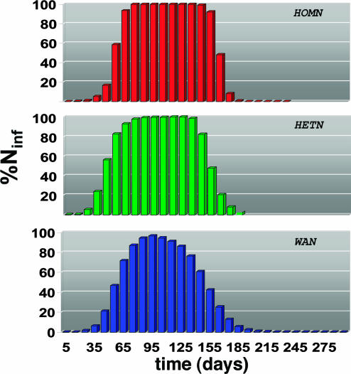
The differences in the behavior observed in the HOMN, the HETN, and the real case provide striking evidence for a direct relation between the network structure and the epidemic pattern. The homogeneous network displays a homogeneous evolution (with H ≈ 1) of the epidemics during a long time window, with sharp changes at the beginning and the end of the spread. We observe a different scenario for heterogeneous networks where H is significantly smaller than one most of the time, with long tails signaling a long lasting heterogeneity of the epidemic behavior. Indeed, the analytical inspection of the epidemic equations points out that the broad variability of the contact pattern (degree distribution) and the ratios w_ij/N_j play an important role in the heterogeneity of the spreading pattern (see the supporting information, which is published on the PNAS web site). Strikingly, the curves obtained for both the real network and the HETN are similar, indicating that, in the case of the airport network, the broad nature of the degree distribution determines to a large extent the overall properties of the epidemic pattern. Fig. 3B reports the average entropy profile together with the maximal dispersion obtained for the spreading starting from a given city with different realizations of the noise. It is clear that the noise has a mild effect and that the average behavior of the entropy is representative of the behavior obtained in each realization. In Fig. 4, we show the percentage of infected cities as a function of time for each null model and for the real case. Although the HOMN displays a long time window in which all cities are infected, this interval is much smaller in the HETN and completely absent in the WAN.

Fig. 4.

Percentage of infected cities as a function of time for an epidemics starting in Hong Kong based on a SIR dynamics within each city. The HOMN case displays a large interval in which all cities are infected. The HETN and the real case show a smoother profile with long tails, signature of a long lasting geographical heterogeneity of the epidemic diffusion.

Predictability and Forecast Reliability.

A further major question in the modeling of global epidemics consists in providing adequate information on the reliability of the obtained epidemic forecast; i.e., the epidemic predictability. Indeed, the intrinsic stochasticity of the epidemic spreading will make each realization unique, and reasonable forecast can be obtained only if all epidemics outbreak realizations starting with the same initial conditions and subject to different noise realizations are reasonably similar. A convenient quantity to monitor in this respect is the vector π⃗(t), whose components are π_j(t) = I_j(t)/Σ_lI_l; i.e., the normalized probability that an infected individual is in city j. The similarity between two outbreaks realizations is quantitatively measured by the statistical similarity of two realizations of the global epidemic characterized by the vectors π⃗^I and π⃗^II, respectively. As a measure of statistical similarity sim(π⃗^I,π⃗^II), we have considered the standard Hellinger affinity π⃗^I and π⃗^II = Σ_j $\sqrt{A}$, $\sqrt{{\pi }_j^I{\pi }_j^{\mathrm{II}}}$. Normalized similarity measures do not account for the difference in the total epidemic prevalence, and we have to consider also sim(i⃗^I, i⃗^II), where i⃗^I(II) = (i^I(II), − i^I(II)) and i(t) = Σ_jI_j(t)/N is the worldwide epidemic prevalence (N = Σ_jN_j is the total population). We can thus define the overlap function measuring the similarity between two different outbreak realizations as

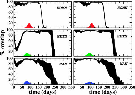
The overlap is maximal [Θ(t) = 1] when the very same cities have the very same number of infectious individuals in both realizations, and Θ(t) = 0 if the two realizations do not have any common infected cities at time t. Clearly, a large overlap corresponds to a predictable evolution, providing a direct measure of the reliability of the epidemic forecast. In the HOMN, we find a significant overlap [Θ(t) > 80%; see Fig. 5] even at the early stage of the epidemics, the most relevant phase for epidemic surveillance. The picture is different if we consider the HETN and the real airport network where especially at the initial stage of the epidemics the predictability is much smaller. These results may be rationalized by relating the level of predictability to the presence of a backbone of dominant spreading channels defining specific “epidemic pathways” that are weakly affected by the stochastic noise. Epidemic pathways are the outcome of the conflict between two different properties of the network. On the one hand, the heterogeneity of the connectivity pattern provides a multiplicity of equivalent channels for the travel of infected individuals depressing the predictability of the evolution. On the other hand, the heterogeneity of traffic flows introduces dominant connections that select preferential pathways increasing the epidemic predictability. The heterogeneous connectivity pattern of the HETN and the WAN thus generates a multiplicity of channels that decreases the predictability. In the real case, the lowering of the epidemic predictability also indicates the dominant effect of the topological heterogeneity that wins over the opposite tendency of the traffic heterogeneity. The above framework is confirmed by the two distinct behaviors depending on the degree of the initial infected city. Epidemics starting in initial cities with a hub airport generate realizations whose overlap initially decreases to 50–60% because of the many possible equivalent paths resulting in a larger differentiation of the epidemic history in each stochastic realization. On the contrary, outbreaks from poorly connected initial cities display a large overlap due to the few available connections that favor the selection of specific epidemic pathways.

Fig. 5.

Percentage of overlap as a function of time. The shaded area corresponds to the standard deviation obtained with 5·10³ couples of different realizations of the global spreading model based on a SIR dynamics within each city. Topological heterogeneity plays a dominant role in reducing the overlap in the early stage of the epidemics. We observe two different behaviors depending on the degree of the initially infected city: a reduced initial predictability in the case of airport hubs (Left) with respect to poorly connected cities (Right). Large fluctuations at the end of the epidemics are observed in the HETN and in the real case, due to the different lifetime of the epidemics in distinct realizations induced by the heterogeneity of the network. We also report the prevalence profile as a function of time showing that the maximum predictability corresponds to a prevalence peak.

Conclusions

From our study, it emerges that the air-transportation-network properties are responsible for the global pattern of emerging diseases. In this perspective, the complex features characterizing this network are the origin of the heterogeneous and seemingly erratic spreading on the global scale of diseases such as severe acute respiratory syndrome. The analysis provided here show that large-scale mathematical models that take fully into account the complexity of the transportation matrix can be used to obtain detailed forecast of emergent disease outbreaks. We have also shown that it is possible to provide quantitative measurements of the predictability of epidemic patterns, providing a tool that might be used to obtain confidence intervals in epidemic forecast and in the risk analysis of containment scenarios. It is clear that to make the forecast more realistic, it is necessary to introduce more details in the disease dynamics. In particular, seasonal effects and geographical heterogeneity in the basic transmission rate (due to different hygienic conditions and health care systems in different countries) should be addressed. Finally, the interrelation of the air transportation network with other transportation systems such as railways and highways could be very useful for forecast on longer time scales. We believe, however, that the basic understanding of the interplay of the transportation network complex features with the disease spreading evolution and the detailed modeling obtained by the full consideration of these features may represent a valuable tool to test traveling restrictions and vaccination policies in the case of new pandemic events.

Materials and Methods

Transport Operator.

The number of passengers of each category traveling from a city j to a city l is an integer random variable, in that each of the X_j^[m] potential travelers has a probability p_jl = w_jlΔt/N_j to go from j to l in the time interval Δt. In each city j, the numbers of passengers ζ_jl traveling on each connection j → l at time t define a set of stochastic variables which follow the multinomial distribution

where (X_j^[m] − Σ_lζ_jl) identifies the number of nontraveling individuals, and we use standard numerical subroutines to generate random numbers of travelers following these distributions.

The transport operator in each city j is therefore written as

where the mean and variance of the stochastic variables are 〈ζ_jl(X_j^[m])〉 = p_jlX _j^[m] and Var(ζ_jl(X_j^[m])) = p_jl(1 − p_jl)X_j^[m]. In addition, since the traffic flows are expressed as the number of available seats on a given connection, we have to consider that the transport operator is in general affected by fluctuations due to an occupancy rate of the airplanes not equal to 1. This introduces a further source of noise because we have to consider that on each connection (j, l), the flux of passengers at each time t is given by a stochastic variable

where α = 0.7 corresponds to the average occupancy rate of 70% provided by official statistics (www.iata.org) and η is a random number drawn uniformly in the interval [−1, 1] at each time step.

Infection Dynamics.

The dynamics of the individuals X^[m] between the different compartments depends on the specific disease considered. In compartmental models, there are two possible elementary processes ruling the disease dynamics. The first class of process refers to the spontaneous transition of one individual from one compartment [m] to another compartment [h]. Processes of this kind are the spontaneous recovery of infected individuals (I → R) or the passage from a latent condition to an infectious one (L → I) after the incubation period. In this case, the variation in the number of individuals X^[m] is simply given by Σ_hv_h^ma_h X^[h], where a_h is the rate of transition from the state [h] and v_h^m ∈ {−1, 0, 1} is the change in the number of X^[m] due to the spontaneous process from or to the compartment [h]. The second class of processes refers to binary interaction among individuals such as the contagion of one susceptible in interaction with an infectious (S + I → 2I). In the homogeneous assumption, the rate of variation of individuals X^[m] is given by Σ_h,g v_h,g^ma_h,gN⁻¹X^[h]X^[g], where a_h,g is the rate of transition rate of the process and v_h,g^m ∈ {−1, 0, 1} is the change in the number of X^[m] due to the interaction. The factor N⁻¹, where N is the number of individuals, stems from the fact that the above expression considers the homogeneous approximation in which the probability for each individual of state [h] to interact with an individual of state [g] is simply proportional to the density X^[g]/N of such individuals [note that it is, however, possible to consider other cases (1)].

Stochastic Formulation of the Global Spreading Model.

To go beyond the usual deterministic approximations, in each city we work directly with the master equations for the processes described above (22); and under the assumption of large populations, we obtain the Langevin equations in which we associate to each reaction process a noise term with amplitude proportional to the square root of the reaction term (26–28). The epidemic Langevin equations are coupled among them by the stochastic transport operator that describes movements of individuals from one city to another and can be numerically solved by considering the discretized evolution equations (26–28) for small time steps Δt that read

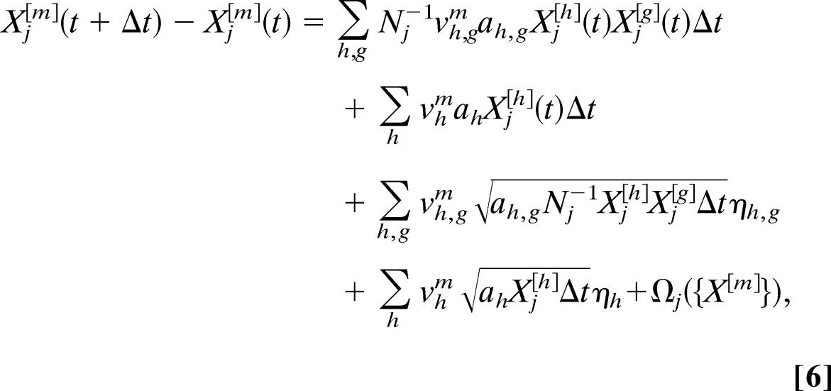where η_h,g and η_h are statistically independent Gaussian random variables with zero mean and unit variance and Θ_j({X}) is the stochastic travel operator (defined in the previous paragraph) depending on the traveling probabilities (obtained from the International Air Transport Association data set) p_jl = w_jlΔt/N_j. The model is thus a compartmental system of differential equations that can be numerically integrated. It is worth mentioning, however, that the standard integration of these equations by using Cauchy–Euler methods leads to a well known technical problem, and specific techniques must be used to avoid an asymmetric truncation of the noise terms (29). A detailed discussion of the integration procedure may be found in the supporting information. In the case of the SIR model used in the article, by considering the three compartments S, I, and R in Eq. 6 and plugging in a_I,S = β, a_I = a_R = μ, and the corresponding parameters v_I,S^I = 1 and v_I^R = −v_I^I = 1, it is possible to obtain explicitly (see the supporting information) the 3,100 × 3 differential equations whose integration provides the disease evolution in every urban areas corresponding to an airport.

Glossary

Abbreviations:

SIR

susceptible–infected–removed.

References

- 1.Anderson R. M., May R. M. Infectious Diseases in Humans. Oxford: Oxford Univ. Press; 1992. [Google Scholar]
- 2.Hethcote H. W., Yorke J. A. Lect. Notes Biomath. 1984;56:1–105. [Google Scholar]
- 3.Kretzschmar M., Morris M. Math. Biosci. 1996;133:165–195. doi: 10.1016/0025-5564(95)00093-3. [DOI] [PubMed] [Google Scholar]
- 4.Keeling M. Proc. R. Soc. London Ser. B; 1999. pp. 859–867. [Google Scholar]
- 5.Pastor-Satorras R., Vespignani A. Phys. Rev. Lett. 2001;86:3200–3203. doi: 10.1103/PhysRevLett.86.3200. [DOI] [PubMed] [Google Scholar]
- 6.Lloyd A. L., May R. M. Science. 2001;292:1316–1317. doi: 10.1126/science.1061076. [DOI] [PubMed] [Google Scholar]
- 7.Meyers L. A., Pourbohloul B., Newman M. E. J., Skowronski D. M., Brunham R. C. J. Theor. Biol. 2005;232:71–81. doi: 10.1016/j.jtbi.2004.07.026. [DOI] [PMC free article] [PubMed] [Google Scholar]
- 8.Ferguson N. M., Keeling M. J., Edmunds W. J., Gani R., Grenfell B. T., Anderson R. M., Leach S. Nature. 2003;425:681–685. doi: 10.1038/nature02007. [DOI] [PMC free article] [PubMed] [Google Scholar]
- 9.Chowell G., Hyman J. M., Eubank S., Castillo-Chavez C. Phys. Rev. E. 2003;68:066102. doi: 10.1103/PhysRevE.68.066102. [DOI] [PubMed] [Google Scholar]
- 10.Eubank S., Guclu H., Anil Kumar V. S., Marathe M. V., Srinivasan A., Toroczkai Z., Wang N. Nature. 2004;429:180–184. doi: 10.1038/nature02541. [DOI] [PubMed] [Google Scholar]
- 11.Albert R., Barabasi A.-L. Rev. Mod. Phys. 2000;74:47–97. [Google Scholar]
- 12.Dorogovtsev S. N., Mendes J. F. F. Evolution of Networks: From Biological Nets to the Internet and WWW. Oxford: Oxford Univ. Press; 2003. [Google Scholar]
- 13.Pastor-Satorras R., Vespignani A. Evolution and Structure of the Internet: A Statistical Physics Approach. Cambridge, U.K.: Cambridge Univ. Press; 2003. [Google Scholar]
- 14.Cohen M. L. Nature. 2000;406:762–767. doi: 10.1038/35021206. [DOI] [PubMed] [Google Scholar]
- 15.Cliff A., Haggett P. Br. Med. Bull. 2004;69:87–99. doi: 10.1093/bmb/ldh011. [DOI] [PubMed] [Google Scholar]
- 16.Rvachev L. A., Longini I. M. Math. Biosci. 1985;75:3–22. [Google Scholar]
- 17.Baroyan O. V., Genchikov L. A., Rvachev L. A., Shashkov V. A. Bull. Int. Epidemiol. Assoc. 1969;18:22–31. [Google Scholar]
- 18.Longini I. M. Math. Biosci. 1988;90:367–383. [Google Scholar]
- 19.Grais R. F., Hugh Ellis J., Glass G. E. Eur. J. Epidemiol. 2003;18:1065–1072. doi: 10.1023/a:1026140019146. [DOI] [PubMed] [Google Scholar]
- 20.Grais R. F., Hugh Ellis J., Kress A., Glass G. E. Health Care Manage. Sci. 2004;7:127–134. doi: 10.1023/b:hcms.0000020652.38181.da. [DOI] [PubMed] [Google Scholar]
- 21.Flahault A., Valleron A. J. Math. Popul. Studies. 1991;3:1–11. [Google Scholar]
- 22.Hufnagel L., Brockmann D., Geisel T. Proc. Natl. Acad. Sci. USA. 2004;101:15124–15129. doi: 10.1073/pnas.0308344101. [DOI] [PMC free article] [PubMed] [Google Scholar]
- 23.Barrat A., Barthélemy M., Pastor-Satorras R., Vespignani A. Proc. Natl. Acad. Sci. USA. 2004;101:3747–3752. doi: 10.1073/pnas.0400087101. [DOI] [PMC free article] [PubMed] [Google Scholar]
- 24.Guimerà R., Mossa S., Turtschi A., Amaral L. A. N. Proc. Natl. Acad. Sci. USA. 2005;102:7794–7799. doi: 10.1073/pnas.0407994102. [DOI] [PMC free article] [PubMed] [Google Scholar]
- 25.Zipf G. K. Human Behavior and the Principle of Least Efforts. Reading, MA: Addison–Wesley; 1949. [Google Scholar]
- 26.Gardiner W. C. Handbook of Stochastic Methods for Physics, Chemistry and Natural Sciences. 3rd Ed. Berlin: Springer; 2004. [Google Scholar]
- 27.Gillespie D. T. J. Chem. Phys. 2000;113:297–306. [Google Scholar]
- 28.Marro J., Dickman R. Nonequilibrium Phase Transitions and Critical Phenomena. Cambridge, U.K.: Cambridge Univ. Press; 1998. [Google Scholar]
- 29.Dickman R. Phys. Rev. E. 1994;50:4404–4409. doi: 10.1103/physreve.50.4404. [DOI] [PubMed] [Google Scholar]
- 30.Gastner M. T., Newman M. E. J. Proc. Natl. Acad. Sci. USA. 2004;101:7499–7504. doi: 10.1073/pnas.0400280101. [DOI] [PMC free article] [PubMed] [Google Scholar]
Associated Data
This section collects any data citations, data availability statements, or supplementary materials included in this article.