Modeling Population Genetic Data in Autotetraploid Species

Abstract

Allozyme and PCR-based molecular markers have been widely used to investigate genetic diversity and population genetic structure in autotetraploid species. However, an empirical but inaccurate approach was often used to infer marker genotype from the pattern and intensity of gel bands. Obviously, this introduces serious errors in prediction of the marker genotypes and severely biases the data analysis. This article developed a theoretical model to characterize genetic segregation of alleles at genetic marker loci in autotetraploid populations and a novel likelihood-based method to estimate the model parameters. The model properly accounts for segregation complexities due to multiple alleles and double reduction at autotetrasomic loci in natural populations, and the method takes appropriate account of incomplete marker phenotype information with respect to genotype due to multiple-dosage allele segregation at marker loci in tetraploids. The theoretical analyses were validated by making use of a computer simulation study and their utility is demonstrated by analyzing microsatellite marker data collected from two populations of sycamore maple (Acer pseudoplatanus L.), an economically important autotetraploid tree species. Numerical analyses based on simulation data indicate that the model parameters can be adequately estimated and double reduction is detected with good power using reasonable sample size.

POLYPLOIDY has played an important role in the evolutionary diversification of up to 80% of angiosperm species (Grant 1971; Lewis 1980; Otto and Whitton 2000; Soltis and Soltis 2000). Two types of polyploids can be distinguished according to their genome origin. Allopolyploids are the product of an interspecific hybridization event and subsequent chromosome doubling, while autopolyploids originate from the whole-genome doubling, likely by fusion of unreduced conspecific gametes. Because bivalents are always formed between pairs of chromosomes with the same origin at meiosis, allopolyploids display disomic inheritance. In contrast, autopolyploids have more than two sets of homologous chromosomes, show multivalent chromosome pairing at meiosis, and display polysomic inheritance. The complexities in modeling polysomic inheritance lie in two major aspects: segregation of multiple dosage alleles at individual loci and the occurrence of double reduction, the phenomenon by which sister chromatids enter into the same gamete (Mather 1936). Another distinct feature in the population genetics of polyploids is the formation of partial heterozygotes. For example, when two alleles (A₁ and A₂) segregate at a locus in an autotetraploid population, there are three types of partial heterozygotes: A₁A₁A₁A₂, A₁A₁A₂A₂, and A₁A₂A₂A₂.

For their significance in evolutionary biology and agriculture, autopolyploids have attracted increasing research efforts at both theoretical and experimental scales (Ronfort et al. 1998; Luo et al. 2000, 2001, 2004; Mahy et al. 2000; Lopez-Pujol et al. 2004). Furthermore, rapid advances in the techniques of molecular biology and computer technology have made the genetical analysis of autopolyploids more tractable than ever before (De Winton and Haldane 1931; Fisher 1947). Allozyme and DNA-based microsatellite markers have been used to investigate the divergent heterozygosity between autotetraploids and their parental diploids (Mahy et al. 2000; Hardy and Vekemans 2001), to infer the genetic mode of autopolyploidy (Lopez-Pujol et al. 2004), and to assess population structure and gene flow in autotetraploid species (Ronfort et al. 1998). Thrall and Young (2000) developed a computer program, AUTOTET, for calculating allele frequencies of genetic markers in autotetraploid populations. However, it must be pointed out that to use the program, one has to empirically infer genotypes of the markers from inspecting the pattern and intensity of electrophoretic gel bands (for example, Lopez-Pujol et al. 2004). Obviously, diagnosing the intensity of gel bands could be unreliable or impossible for the marker data generated, for example, from DNA sequencers.

In this article, we develop a likelihood-based method for calculating allele frequencies of genetic markers in a random-mating autotetraploid population. The method accounts properly for the problem of missing information of marker phenotype in regard to the corresponding genotype and for the presence of double reduction. It can be used to analyze the genetic structure of autotetraploid populations by making use of allozyme and PCR-based molecular markers. The method is demonstrated by analyzing a data set consisting of five microsatellite markers scored on two populations of Acer pseudoplatanus L., an autotetraploid tree species.

THEORY AND METHODS

Model and notation:

We consider segregation of alleles at a locus in a random-mating autotetraploid population. Let L be the number of alleles, A₁, A₂, … , A_L, segregating in the population and the frequencies of the alleles be , respectively. The coefficient of double reduction, which is the probability of sister chromatids ending up in the same gamete in meiosis (Mather 1936), at the marker locus is denoted by α. Geiringer (1949) found that the equilibrium distribution of zygotic genotypes is given by the expansion of

(1)

If α = 0, this is

(2)

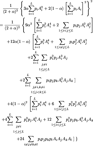
After algebraic simplification, Equation 1 becomes

(3)

It can be seen that there are as many as distinct genotypes at the marker locus (Luo and Ma 2004). To ease the following analysis, we classed the individual genotypes into three groups according to the number of double-reduction gametes they carried and illustrated the equilibrium genotypic distribution in Table 1.

TABLE 1.

The genotypic distribution at a single locus with L alleles in a random mating autotetraploid population

Zygotes	Genotypes	Probabilities	No. of terms
Individuals carrying two DR gametes []
Homozygotes	AiAiAiAi (1 ≤ i ≤ L)		L
Heterozygotes	AiAiAjAj (1 ≤ i < j ≤ L)
Individuals carrying one DR gamete []
Homozygotes	AiAiAiAi (1 ≤ i ≤ L)		L
Heterozygotes	AiAiAiAj (1 ≤ i < j ≤ L)
AiAjAjAj (1 ≤ i < j ≤ L)
AiAiAjAj (1 ≤ i < j ≤ L)
AiAiAjAk (1 ≤ j < k ≤ L)
AiAjAjAk (1 ≤ j < k ≤ L)
AiAjAkAk (1 ≤ j < k ≤ L)
Individuals carrying no DR gamete []
Homozygotes	AiAiAiAi (1 ≤ i ≤ L)		L
Heterozygotes	AiAiAiAj (1 ≤ i < j ≤ L)
AiAiAjAj (1 ≤ i < j ≤ L)
AiAiAjAk (1 ≤ i < j, k ≤ L)
AiAjAjAk (1 ≤ i < j, k ≤ L)
AiAjAkAk (1 ≤ i < j, k ≤ L)
	AiAjAkAl (1 ≤ i < j, k < l ≤ L)

Analysis and statistical inference:

The genotypic distribution involves L independent unknown parameters: since . When the individual genotypes are distinguishable directly from the phenotype data, estimation of the double-reduction and allelic frequency parameters becomes trivial. However, there is no one-to-one relationship between genotype and phenotype at any genetic markers in the autotetraploids (Luo et al. 2000). To estimate the model parameters, one has to work with phenotype data. For simplicity but without loss of generality, we denote the phenotype of an autotetraploid individual at a marker locus by the number of distinct gel bands scored at the marker locus. For a given dominance mode of the markers, it is easy to convert the marker genotype distribution into the corresponding phenotype distribution. For example, the genotype distribution tabulated in Table 1 can be transformed into the phenotype distribution that is summarized in Table 2 when the marker alleles are assumed to display codominant inheritance. It can be seen from Table 2 that a phenotype provides full information of the corresponding genotype only if the phenotype is represented as four distinct bands; i.e., the presence of four different alleles and, in most cases, an individual genotype cannot be inferred directly from the corresponding phenotype. A general form for converting the genotypic distribution (Table 1) into the phenotypic distribution (Table 2) is , where the summation is over all genotypes that correspond to the same phenotype, x = i (one band), ij (two bands), ijk (three bands), or ijkl (four bands). g_h is the probability of genotype h that is compatible with phenotype x. For example, there are three genotypes (A_iA_iA_iA_j, A_iA_iA_jA_j, and A_iA_jA_jA_j) that are compatible with phenotype ij; thus f_ij, the probability of this phenotype, equals as given in Table 2. Let n be the number of individuals randomly sampled from the population under question and m be the number of different phenotypes observed in the sample. 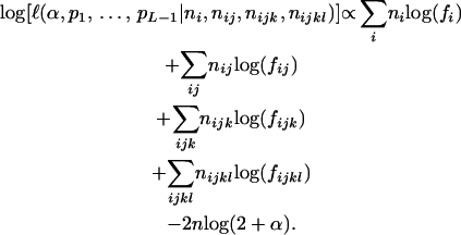The sample can be divided into phenotype groups for which there are n_i, n_ij, , and of individuals with one, two, three, and four bands, accordingly. The logarithm of the likelihood function of the observed phenotype data given the model parameters is given by

(4)

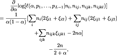
Differentiating Equation 4 with respect to α gives

(5)

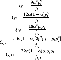
where

(6)

in which f_i, f_ij, and f_ijk are given in Table 2. The maximum-likelihood estimate (MLE) of the unknown parameter, α, can be solved from setting the derivative equation to zero as

(7)

in which . Differentiating Equation 4 with respect to gives

(8)

where

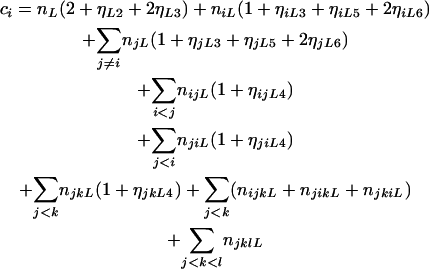(9)

and

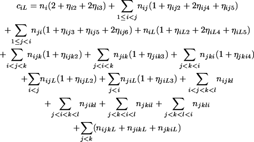(10)

in which

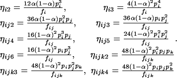(11)

Setting the derivative Equations 8 to equal zero, we obtain L − 1 linear equations in the form of

(12)

where is a square matrix with and , , and . Solving Equation 12 yields the MLEs of allelic frequencies . In fact, Equations 6 and 7 and Equations 11 and 12 represent an EM algorithm for calculating the maximum-likelihood estimates of the model parameters. The algorithm involves iterating the two steps: the expectation step that calculates the posterior probabilities according to Equations 6 and 11 and then the maximization step that calculates the maximum-likelihood estimates of the model parameters from Equations 7 and 12 with ξ's and η's being calculated from the previous expectation step. These two steps are iterated until the sequence of the likelihood function (4) converges. In contrast, the MLEs of marker allele frequencies can be simplified as in diploid populations.

TABLE 2.

The phenotypic distribution at a single locus with L alleles in a random-mating autotetraploid population

Phenotypes (probability)	Form of the probability []	Observations	No. of terms
One band ()		()	L
Two bands ()		()	L(L − 1)/2
Three bands ()		()	L(L − 1)(L − 2)/6
Four bands ()		()	L(L − 1)(L − 2)(L − 3)/24

It is feasible to create a likelihood-based statistical test for the presence of double reduction with the MLEs, . In fact, the test statistic given by

(13)

has an asymptotic chi-square distribution with 1 d.f. and can be used to test the significance of double reduction at the locus under question.

Test for Hardy–Weinberg hypothesis:

The above analysis is based on the assumption that segregation of the marker alleles follows the Hardy–Weinberg equilibrium; i.e., frequencies of marker genotypes are determined by the coefficient of double reduction and the relevant allele frequencies. With the MLEs of the model parameters, the expected genotype (or phenotype) frequencies can be calculated and thus a chi-square statistic with a form of

(14)

can be constructed to test for significance of the hypothesis. It should be pointed out that the number of segregating alleles in the population might be so large for the sample size that the numbers of individuals for most genotype classes are too small for the chi-square test to be reliable. To avoid this problem, we suggest that the expected number of the phenotype classes that is >1 be used to calculate the chi square.

Estimation of genetic heterozygosity:

With the MLEs of the allelic frequencies, one can estimate genetic heterozygosity at marker loci. The genetic heterozygosity, which accounts for the distinct allelic constitutions of tetraploid genotypes, was defined as the probability of any two alleles being not identical in a given genotype (Bever and Felber 1992; Thrall and Young 2000). In the present context and notations, the observed genetic heterozygosity can be calculated from

(15)

whose expectation is given by

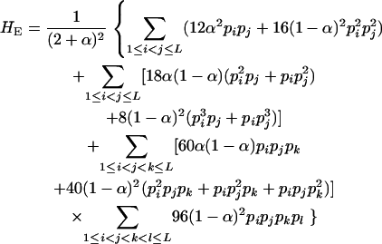(16)

When marker data are collected from k subpopulations of a tetraploid species, one can calculate marker heterozygosity for each of these populations according to the above analysis. Let be the heterozygosity in the subpopulation I, and . We define forms of Wright's F-statistics for autotetraploids by assimilating that in diploids (Hartl and Clark 1997) as

(17)

and

(18)

where and is the expected heterozygosity of an equivalent total population of all the subpopulations under the Hardy–Weinberg equilibrium.

NUMERICAL ANALYSES

Simulation study:

To validate the method presented above and to investigate its properties, we set up a simulation study to mimic segregation of alleles at a single marker locus in autotetraploid populations at equilibrium. The simulation model allows us to vary the number and frequencies of marker alleles and to simulate different values of the coefficient of double reduction. For any given simulated parameters, individual genotypes were randomly sampled from the simulated population for which the genotypic distribution is defined in Table 1. The sampled genotypes were converted into phenotypes according to Luo et al (2000). The simulation study considered the segregation of five marker alleles with either an equal frequency or different frequencies in populations of different sample sizes and two values of the coefficient of double reduction, α = 0.05 and 0.1, at the marker locus.

Tabulated in Table 3 are the means and standard deviations of the MLEs of the coefficient of double reduction and allelic frequencies over 100 repeated simulations, together with the simulation parameters. Also, empirical power, , is listed for detecting significance of double reduction, which was calculated as the proportion of significant tests of double reduction in the repeated simulations. It can be seen from Table 3 that the parameters are estimated adequately in all cases even with a sample size as small as n = 50. Double reduction can be detected with fairly good power when the sample size is not <100 and when α = 0.1. For a given sample size, double reduction is tested with larger power when marker alleles are evenly distributed as compared to noneven distribution of marker alleles. As expected, the standard deviation of the estimates decreases and the power of the double reduction test increases with increasing sample size.

TABLE 3.

Means and corresponding standard deviations (in parentheses) of the maximum-likelihood estimates of simulated coefficient of double reduction, α = 0.05 or 0.1, and allelic frequencies (i = 1, 2, … , 5) over 100 repeated simulations of varying sample sizes, n

n							(%)
50	0.2014 (0.034)	0.1971 (0.033)	0.1988 (0.032)	0.2035 (0.033)	0.1993 (0.031)	0.0586 (0.053)	14
100	0.2012 (0.025)	0.2005 (0.023)	0.2006 (0.024)	0.1968 (0.023)	0.2009 (0.025)	0.0469 (0.035)	12
200	0.2007 (0.017)	0.1981 (0.016)	0.2008 (0.015)	0.1983 (0.017)	0.2021 (0.015)	0.0466 (0.30)	29
50	0.1980 (0.031)	0.1948 (0.031)	0.1972 (0.032)	0.2051 (0.034)	0.2049 (0.032)	0.0954 (0.062)	31
100	0.1980 (0.024)	0.2020 (0.024)	0.1971 (0.025)	0.1989 (0.020)	0.2042 (0.024)	0.0904 (0.045)	54
200	0.1998 (0.017)	0.1990 (0.017)	0.2005 (0.017)	0.2016 (0.017)	0.1991 (0.017)	0.0943 (0.032)	84
50	0.4011 (0.044)	0.3008 (0.039)	0.1929 (0.030)	0.0955 (0.022)	0.0097 (0.006)	0.0523 (0.051)	4
100	0.3999 (0.030)	0.2996 (0.029)	0.1918 (0.020)	0.0992 (0.016)	0.0095 (0.005)	0.0581 (0.040)	10
200	0.4009 (0.023)	0.3007 (0.020)	0.1894 (0.014)	0.0995 (0.013)	0.0095 (0.003)	0.0514 (0.034)	23
50	0.4043 (0.044)	0.2956 (0.046)	0.1872 (0.030)	0.1027 (0.025)	0.0101 (0.007)	0.0979 (0.069)	22
100	0.4026 (0.030)	0.2973 (0.025)	0.1888 (0.022)	0.1013 (0.016)	0.0100 (0.005)	0.0934 (0.054)	44
200	0.4015 (0.023)	0.3022 (0.019)	0.1872 (0.016)	0.0983 (0.011)	0.0109 (0.004)	0.0912 (0.042)	65

is the empirical power of the statistical test for double reduction.

Analysis of microsatellite data from two sycamore maple populations:

Sycamore maple (A. pseudoplatanus L.) is a forest tree species native to central Europe and western Asia, growing especially in mountainous regions. The species is an autotetraploid with a chromosome number of 2n = 4x = 52 (Darlington and Wylie 1955). Because of its economic and ecological importance, numerous plantations were established throughout Europe during the last century. However, the genetic structure and its mating system in natural populations or in plantations remain unclear.

To explore the genetic variation pattern, gene flow, and mating system of the species, Pandey et al. (2004) have started developing microsatellite markers in this species. For a proof-of-principle demonstration purpose, we detailed here analysis of data of a marker, MAP-9, which was scored for 133 and 80 individuals, respectively, from two populations, Södderich and Weisswassertal, near Göttingen in Germany. The marker data, which were collected as peak value reads from the ABI PRISM 3100 genetic analyzer (Applied Biosystems, Foster City, CA/Hitachi, San Jose, CA), were converted into gel-band-like phenotypes.

Table 4 summarizes the phenotypic distribution and analysis of the marker data in the two sycamore maple populations. It shows that the 133 and 80 individuals sampled from the two populations can be grouped into 12 and 6 different phenotypic groups, respectively. From the phenotype, seven distinct marker alleles are observed in the Södderich population sample but only five of these are present in the Weisswassertal population sample. From the data sets, the maximum-likelihood estimates are calculated for frequencies of the marker alleles and the coefficient of double reduction by making use of the method developed in this study. It shows that marker alleles 1 and 3 are detected in the two populations as the most frequently occurring alleles. There is no evidence of double reduction at this marker locus. The goodness-of-fit test demonstrates that segregation of the marker alleles in both the populations agrees well with the Hardy–Weinberg equilibrium (). To make the chi-square-based fitness tests more stable (Kendall and Stuart 1961, p. 440), the analysis has excluded those phenotype classes with expected sample observations <1.0. In addition, we calculated genetic heterozygosity (H_O) at the marker locus using Equation 15 and observed that H_O = 0.6901 and 0.6833 for the Södderich and the Weisswassertal populations, respectively. On the basis of the observed genetic heterozygosity estimates and their corresponding expected values that can be calculated from Equation 16, the F_ST is estimated to be 0.001, suggesting trivial genetic differentiation between the two populations.

TABLE 4.

Summary and analysis of microsatellite marker data collected from two Sycamore maple (Acer pseudoplatanus) populations, Södderich and Weisswassertal

Södderich (n = 133)					Weisswassertal (n = 80)
Phenotype	Obs.	Exp.	Allele and		Phenotype	Obs.	Exp.	Allele and
1 0 1 0 0 0 0	81	67.14	1	0.4390	1 1 0 0 0	49	42.69	1	0.4418
1 0 1 1 0 0 0	27	19.30	2	0.0038	1 1 1 0 0	14	9.20	3	0.4418
1 0 1 0 0 1 0	4	6.72	3	0.4325	1 1 0 1 0	7	6.63	4	0.0525
1 0 1 0 1 0 0	4	5.64	4	0.0678	1 1 0 0 1	5	4.33	5	0.0384
1 1 1 0 0 0 0	2	1.00	5	0.0209	1 1 1 1 0	2	0.76	6	0.0254
1 0 1 0 0 0 1	1	3.02	6	0.0247	1 1 0 1 1	3	0.37
1 0 0 1 0 1 0	1	0.62	7	0.0113
1 0 1 0 1 1 0	6	0.31
1 0 1 1 0 0 1	4	0.46
1 0 1 1 1 0 0	1	0.86
1 0 1 1 0 1 0	1	1.02	= 0.0000		= 0.0001
1 0 1 0 0 1 1	1	0.17	= 9.86					= 3.56

and are the maximum-likelihood estimates of the coefficient of double reduction and frequency of the ith marker allele. The chi-square value, , was calculated by sorting together those phenotype classes whose expected counts were <1.

Obs., observed; Exp., expected.

DISCUSSION

There has been increasing interest in investigating genetic diversity and population genetic structure of autotetraploid species for understanding evolutionary impacts of polyploidy and the conservation biology of the species (Brown and Young 2000; Mahy et al. 2000; Hardy and Vekemans 2001; Lopez-Pujol et al. 2004). This has been greatly promoted by the increasing availability of allozyme and PCR-based DNA molecular marker data in these populations. However, analysis of the fast growing data sets of DNA polymorphic markers raises challenges to the development of appropriate statistical methods and algorithms. The data sets have been analyzed by empirically inferring individual genotype from the intensity of gel bands (Soltis and Soltis 1989; Wendel and Weeden 1989; Lopez-Pujol et al. 2004). It is well known that this will be either inaccurate or unfeasible for most PCR-based DNA markers. Thus, development of theory and methods for modeling and analyzing these data sets meets the urgent needs of the research area.

This article developed a theoretical model for characterizing genetic segregation of alleles at genetic marker loci, an autotetraploid population locus and a novel maximum-likelihood-based method to estimate the parameters defining the population genetic model. The model properly accounts for segregation complexities due to multiple alleles and double reduction at tetrasomic loci in natural populations, and the statistical method takes appropriate account of incomplete marker phenotype information with respect to the genotype due to multiple dosage allele segregation at marker loci in tetraploids. The theoretical analysis and methods developed in this study are validated by making use of a computer simulation study and their utility is demonstrated by analyzing microsatellite marker data collected from two populations of sycamore maple (A. pseudoplatanus L.), an economically important autotetraploid tree species. Numerical analyses based on simulation data indicate that the model parameters can be adequately estimated and double reduction is detected with good power with a sample size of ∼100. Analysis of the sycamore maple data illustrates the data format required by the statistical method and demonstrates how the method can be used to predict various population genetic parameters by using DNA molecular data in autotetraploid species. A practical problem in real data analysis might be that the number of segregating alleles is too large in relation to reasonable sample sizes. Thus, the sample size required for accurate parameter estimation and efficient testing of double reduction may depend largely on the number of segregating alleles; the sample size considered here may be suitable only when there are several marker alleles segregating in the population.

Although the theory and methods developed in this study were demonstrated for codominant markers, it is feasible for their extension to dominant markers such as RAPDs, AFLPs, etc. In fact, there are usually two segregating alleles at these marker loci, i.e., a dominant and a recessive allele; this greatly reduces the number of possible genotypes and the number of possible phenotypes at the locus and thus simplifies the model. In addition, the recessive allele will be phenotypically present only when it is present in four copies.

Double reduction is one of the most distinguished features of tetrasomic inheritance and also one of the major difficulties in modeling tetrasomic inheritance when compared to disomic inheritance. Butruille and Boiteux (2000) exploited the impact of double reduction on the evolution of deleterious mutants in autotetraploid genomes and found that low frequencies of double reduction are enough to reduce equilibrium frequencies, which are maintained at a selection and mutation balance, by severalfold. This suggests the important effect of double reduction on the evolution of the species. However, there are no proposals, either in their study or in the literature, to address how to test for the significance of double reduction in natural populations of the species. This study provides such a test and thus fills a gap in the evolutionary study of autotetraploid species.

The algorithm developed in this study was programmed in Fortran-90 computer language. The program is available upon request from the corresponding author.

References

- Bever, J. D., and F. Felber, 1992. The theoretical population genetics of autopolyploidy, pp. 185–217 in Oxford Surveys in Evolutionary Biology, edited by J. Antonovics and D. Futuyma. Oxford University Press, Oxford.
- Brown, A. H. D., and A. G. Young, 2000. Genetic diversity in tetraploid populations of the endangered daisy Rutidosis leptorrhynchoides and implications for its conservation. Heredity 85: 122–129. [DOI] [PubMed] [Google Scholar]
- Butruille, D. V., and L. S. Boiteux, 2000. Selection-mutation balance in polysomic tetraploids: impact of double reduction and gametophytic selection on the frequency and subchromosomal localization of deleterious mutations. Proc. Natl. Acad. Sci. USA 97: 6608–6613. [DOI] [PMC free article] [PubMed] [Google Scholar]
- Darlington, C. D., and A. P. Wylie, 1955. Chromosome Atlas of Flowering Plants. George Allen & Unwin, London.
- De Winton, D., and J. B. S. Haldane, 1931. Linkage in the tetraploid Primula sinensis. J. Genet. 24: 121–144. [Google Scholar]
- Fisher, R. A., 1947. The theory of linkage in polysomic inheritance. Philos. Trans. R. Soc. Lond. B 233: 55–87. [Google Scholar]
- Geiringer, H., 1949. Chromatid segregation in tetraploids and hexaploids. Genetics 34: 665–684. [DOI] [PMC free article] [PubMed] [Google Scholar]
- Grant, V., 1971. Plant Speciation. Columbia University Press, New York/London.
- Hardy, O. J., and X. Vekemans, 2001. Patterns of allozyme variation in diploid and tetraploid Centaurea jacea at different spatial scales. Evolution 55: 943–954. [DOI] [PubMed] [Google Scholar]
- Hartl, D. H., and A. G. Clark, 1997. Principles of Population Genetics, Ed. 3. Sinauer Associates, Sunderland, MA.
- Kendall, M. G., and A. Stuart, 1961. The Advanced Theory of Statistics: Inference and Relationship, Vol. 2. Charles Griffin, London.
- Lewis, W. H., 1980. Polyploidy: Biological Relevance. Plenum Press, New York.
- Lopez-Pujol, J., M. Bosch, J. Simon and C. Blanche, 2004. Allozyme diversity in the tetraploid endemic Thymus loscossi (Lamiaceae). Ann. Bot. 93: 323–332. [DOI] [PMC free article] [PubMed] [Google Scholar]
- Luo, Z. W., and L. Ma, 2004. An improved formulation of marker heterozygosity in recurrent selection and backcross schemes. Genet. Res. 83: 49–53. [DOI] [PubMed] [Google Scholar]
- Luo, Z. W., C. A. Hackett, J. E. Bradshaw, J. W. McNicol and D. Milbourne, 2000. Predicting parental genotypes and gene segregation for tetrasomic inheritance. Theor. Appl. Genet. 100: 1067–1073. [Google Scholar]
- Luo, Z. W., C. A. Hackett, J. E. Bradshaw, J. W. McNicol and D. Milbourne, 2001. Construction of a genetic linkage map in tetraploid species using molecular markers. Genetics 157: 1369–1385. [DOI] [PMC free article] [PubMed] [Google Scholar]
- Luo, Z. W., R. M. Zhang and M. J. Kearsey, 2004. Theoretical basis for genetic linkage analysis in autotetraploid species. Proc. Natl. Acad. Sci. USA 101: 7040–7045. [DOI] [PMC free article] [PubMed] [Google Scholar]
- Mahy, G., L. P. Bruederle, B. Connors, M. Van Hofwegen and N. Vorsa, 2000. Allozyme evidence for genetic autopolyploidy and high genetic diversity in tetraploid cranberry, Vaccinium oxycoccos (Ericaceae). Am. J. Bot. 87: 1882–1889. [PubMed] [Google Scholar]
- Mather, K., 1936. Segregation and linkage analysis in autotetraploids. J. Genet. 32: 287–314. [Google Scholar]
- Otto, S. P., and J. Whitton, 2000. Polyploid incidence and evolution. Annu. Rev. Genet. 34: 401–437. [DOI] [PubMed] [Google Scholar]
- Pandey, M., O. Gailing, D. Fischer, H. H. Hattemer and R. Finkeldey, 2004. Characterization of microsatellite markers in sycamore (Acer pseudoplatanus L.). Mol. Ecol. Notes 4: 253–255. [Google Scholar]
- Ronfort, J., E. Jenczewski, T. Bataillon and F. Rousset, 1998. Analysis of population structure in autotetraploid species. Genetics 150: 921–930. [DOI] [PMC free article] [PubMed] [Google Scholar]
- Soltis, D. E., and P. S. Soltis, 1989. Genetic consequences of autopolyploidy in Tolmiea (Saxifragaceae). Evolution 43: 586–594. [DOI] [PubMed] [Google Scholar]
- Soltis, P. S., and D. E. Soltis, 2000. The role of genetic and genomic attributes in the success of polyploids. Proc. Natl. Acad. Sci. USA 97: 7051–7057. [DOI] [PMC free article] [PubMed] [Google Scholar]
- Thrall, P. H., and A. Young, 2000. AUTOTET: a program for the analysis of autotetraploid genotypic data. J. Hered. 91: 348–349. [DOI] [PubMed] [Google Scholar]
- Wendel, F., and N. F. Weeden, 1989. Visualization and interpretation of plant isozymes, pp. 5–45 in Isozymes in Plant Biology, edited by D. E. Soltis and P. S. Soltis. Dioscorides Press, Portland, OR.