Abstract
The identification of genes in the human genome remains a challenge, as the actual predictions appear to disagree tremendously and vary dramatically on the basis of the specific gene-finding methodology used. Because the pattern of conservation in coding regions is expected to be different from intronic or intergenic regions, a comparative computational analysis can lead, in principle, to an improved computational identification of genes in the human genome by using a reference, such as mouse genome. However, this comparative methodology critically depends on three important factors: (1) the selection of the most appropriate reference genome. In particular, it is not clear whether the mouse is at the correct evolutionary distance from the human to provide sufficiently distinctive conservation levels in different genomic regions, (2) the selection of comparative features that provide the most benefit to gene recognition, and (3) the selection of evidence integration architecture that effectively interprets the comparative features. We address the first question by a novel evolutionary analysis that allows us to explicitly correlate the performance of the gene recognition system with the evolutionary distance (time) between the two genomes. Our simulation results indicate that there is a wide range of reference genomes at different evolutionary time points that appear to deliver reasonable comparative prediction of human genes. In particular, the evolutionary time between human and mouse generally falls in the region of good performance; however, better accuracy might be achieved with a reference genome further than mouse. To address the second question, we propose several natural comparative measures of conservation for identifying exons and exon boundaries. Finally, we experiment with Bayesian networks for the integration of comparative and compositional evidence.
Computational gene identification systems have made tremendous progress in the last twenty years and have been reviewed by M.Q. Zhang and many other authors (Burset and Guigo 1996; Fickett 1996; Gelfand et al. 1996; Kulp et al. 1996; Claverie 1997, 1998; Krogh 1997; Zhang 1997, 2002; Birney and Durbin 2000; Parra et al. 2000; Rogic et al. 2001; http://linkage.rockefeller.edu/wli/gene; http://www.cbc.umn.edu/ResearchProjects/BIBLIOGRAPHY/gene_finding/gene_finding.html). However, exact identification of genes in the human genome remains a challenge, as the estimates on the number of human genes and their precise boundaries vary dramatically, depending on the specific gene-finding methodology used (Crollius et al. 2000; Ewing and Green 2000; Liang et al. 2000). The limited ability to identify human genes results in substantial disparities in genome annotation, as documented by the comparison of the human genome annotations predicted by Celera and Ensembl (Hogenesch et al. 2001). In fact, 80% of the novel transcripts were predicted by only one of the two groups.
The advent of whole-genome sequencing creates a starting point for cross-species comparative analysis that provides unprecedented opportunities to identify the evolutionary roadmap leading to a better understanding and classification of DNA sequences (Lander et al. 2001; Venter et al. 2001; Mural et al. 2002). Additionally, genomic comparative analyses can exploit the variable rate of conservation of different functional regions and provide us with additional evidence that can assist in genomic annotation and gene identification. It is expected that intergenic regions might be characterized by low conservation, whereas protein-coding regions might exhibit a higher conservation rate that depends on the specific function of the protein. A comparative gene-identification system can take advantage of the selective evolutionary pressures that result in different conservation rates in different genomic regions to produce a more accurate identification of functional genomic regions, such as protein-encoding exons. Such regions are expected to have higher conservation rates (on average) than intergenic regions, and the pattern of substitutions is expected to obey a synonymous/nonsynonymous rate that is not expected in introns or other noncoding regions.
In anticipation of the full sequencing of the complete mouse genome sequence (Waterston et al. 2002), several systems have been built with the goal of identifying genes in the human genomic sequences using human–mouse comparative evidence (Batzoglou et al. 2000; Korf et al. 2001; Yeh et al. 2001; Pachter et al. 2002; Parra et al. 2003). Although these systems have achieved reasonably good performance, there are several fundamental questions still open in the comparative identification of human genes. The first key scientific problem is the choice of the reference genome for human gene identification. The mouse genome is generally believed to be a good reference, because most human genes have mouse counterparts, and the evolutionary time between human and mouse seems to be appropriate. In this study, we propose a general computational model to characterize the correlation of the prediction performance and the evolutionary distance between genomes. We then investigate the same correlation with our comparative gene-prediction system. Our results show a reasonable range of organisms at different evolutionary times that, on average, are likely to deliver comparable performance for gene identification. This is the first study that provides a clear link between evolutionary time and performance of gene recognizers.
The second question to address is the choice of comparative features used to assist in comparative gene recognition. We introduce the idea of comparative consensus models for splice sites, translational initiation, and termination sites. In addition, we describe and analyze a variety of discriminative comparative features for identifying coding and noncoding regions and evaluate their performance with a comparative gene-prediction model.
The final question to address is the choice of the evidence integration model for effective gene recognition. There are generally four related, but technically different types of architectures that should provide good performance, for example, Bayesian Networks (Pavlovic et al. 2002), Product-HMMs (Hidden Markov Model) (Walker et al. 2002), Generalized HMMs (Korf et al. 2001; Yeh et al. 2001), and Pair-HMMs/Generalized Pair-HMMs (Pachter et al. 2002). Here, we demonstrate the integration of different sources of evidence with the Bayesian network models. In a subsequent study, we will describe the application of Product-HMMs to comparative gene recognition.
METHODS
Data Set
Part of the data used in this study is based on Batzoglou's set of 117 human–mouse orthologs reported in Batzoglou et al. (2000). A total of 20 of the 117 ortholog pairs containing ambiguous annotations or particularly short intergenic sequences (<100 nucleotides) were discarded. The remaining 97 human sequences are used as our data set for comparative analysis and model training, and their corresponding mouse orthologs are deployed as reference sequences. To compare our prediction system with some available gene finders, IMOG (15 pairs of single-gene sequences) and BI (3 pairs of multi-gene sequences) data sets from SGP2 (Parra et al. 2003) data set were used as the benchmark. One pair of sequences (MT3) from IMOG data set and one pair of sequences (HOX) from BI data set are discarded because of ambiguous bases in the sequences. To document the prediction performance, annotations available for the human sequences are contrasted with our comparative predictions. The annotations of mouse sequences are generally ignored in our analysis.
Each of the human and mouse ortholog pairs is aligned by a global alignment system, GLASS, described in Batzoglou et al. (2000). We characterize the GLASS alignment using a Human Comparative Indicator Sequence or HCIS. The HCIS is, in essence, the output of the global alignment given by a binary sequence with the same length as that of the corresponding human sequence, as shown in Figure 1. At each position in the human sequence, a 1 or 0 in the HCIS indicates a match or a mismatch/gap in the alignment. Our HCIS is similar to, but different from the conservation sequences in the TWINSCAN model, in that TWINSCAN treats gaps and mismatches differently (Korf et al. 2001). The 97 human sequences from Batzoglou's set are also aligned against a mouse peptide database, downloaded from Ensembl (Hubbard et al. 2002), using BLASTX (Altschul et al. 1997).
Figure 1.
Illustration of the GLASS alignment of human and mouse orthologs, Human Comparative Indicator Sequence (HCIS), and base scores for local windows of length 5. HCIS is essentially the output of the global alignment system. It is defined as a binary sequence with 1 indicating a match and 0 a mismatch/gap in the alignment. LBS/RBS at position i is the number of matches in the local window of length k (5 in the example, 20–30 in the study) that ends/starts at position i.
Comparative Analysis
Our proposed comparative evidence includes the following families of comparative models: (1) conservation models for coding and noncoding regions, (2) translational initiation/termination models, and (3) splice site models. These models depend on various comparative statistics obtained from the alignment of the sequences (both global and local). In fact, to compute a local comparative score (see below), we first need to rely on an approximate global alignment. Once such an alignment is available, we can obtain local comparative scores by aligning specific local windows in both sequences to obtain more refined information about their alignment.
Human–Mouse Comparative Features
Three comparative local scores were constructed to measure the degree of conservation between human and mouse as follows: (1) a base-level score, (2) a TBLASTX-based score, and (3) a score from BLASTX analysis with mouse peptide matches. We also introduced additional discrimination between coding and noncoding regions using mathematical transformations of the HCIS, a Fourier transform, and a run-length-encoding representation.
Base Scores
The base-level score measures local conservation in the alignment of orthologs, as defined by the HCIS. At each position in the GLASS alignment, the left base score (LBS) and the right base score (RBS) measure the number of matches in the left and right subsequences of specific lengths flanking the position. The LBS/RBS scores are computed in windows of length 20–30. Figure 1 demonstrates an example of the base scores with a window length five.
TBLASTX Scores
Although indicative of different genomic regions, base-level scores rely on the conservation of individual bases rather than codons, a method that may be preferential for coding regions. The second type of score, the TBLASTX comparative score, attempts to alleviate this problem. Two types of TBLASTX scores, phase-dependent and phase-independent TBLASTX scores, are defined. At each position in the human sequences, the left/right subsequence (of specific length) flanking this position was aligned against the corresponding mouse left/right subsequence (of the same length) by NCBI TBLASTX6 (Altschul et al. 1997). For instance, with the same alignment as shown in Figure 1, the left and right subsequences flanking human position i are GGCGC and CTGAG, by assuming the window of length 5. Their corresponding mouse subsequences in the alignment are AGCCC and CCAGG. A window of length 60–100 was used in our study and bitscores were recorded. Bitscores measure the significance of the conservation on protein level and provide information related to synonymous/nonsynonymous rates in coding regions. Because each TBLASTX alignment considers six different frame-orientation combinations, the comparative TBLASTX score has a potential to depend on the phase (coding frame) as well. Hence, the phase-independent TBLASTX score is given by the maximum of the bitscores recorded, whereas the phase-dependent TBLASTX score with phase j, j ε {0,1,2} is the maximum of HSP (High Scoring Pair) scores with phase j at human position i.
BLASTX Scores
To demonstrate the capability of the system to integrate a wide range of evidence, we designed BLASTX scores based on the BLASTX analysis. Each of the human genomic sequences was aligned against the mouse peptide database with BLASTX (default NCBI BLAST parameters used). At those positions in the human genomic sequences that are not covered by any HSP in the alignment, the corresponding BLASTX scores are defined as zeros. If a position is covered by more than one HSP, the BLASTX score at the position becomes the maximum of the bitscores of the covering HSPs.
Additional Comparative Features
In addition to these comparative scores, two other comparative features were analyzed that measure characteristics of the distributions of 1s and 0s in the HCIS. One is the run-length distribution of contiguous 1s in the HCIS, and the other is a Fourier analysis of the HCIS. The run-length analysis characterizes the distribution of the lengths of matches in different genomic regions. The Fourier score, on the other hand, measures the periodicity of matches or mismatches/gaps in the alignment. Both features attempt to amplify a characteristic related to the positions of synonymous changes in coding regions—usually, substitutions of the third base of a codon are synonymous and occur more frequently.
Analysis of Human–Mouse Comparative Scores
Although most comparative scores would rarely be used in isolation from other genomic features for gene identification, their own capacity to distinguish coding from noncoding sequences may be a good initial indication of their overall utility. One common way to analyze the prediction performance of these scores is Receiver Operating Characteristic (ROC) analysis (Egan 1975). ROC analysis demonstrates the correlation of the sensitivity (SN) and specificity (SP) of the predictions made by each comparative score. We assume that predictions are made using a likelihood ratio test:
 |
in which scorei is one of the proposed comparative scores evaluated at position i in a human sequence. Likelihood distributions are estimated from our data set of orthologs. The predictions are then compared with the annotations, and the SN and SP are evaluated by
 |
in which TP, FN, TN, and FP stand for true positive, false negative, true negative, and false positive, respectively. As the threshold changes, the corresponding SN and SP vary and an ROC curve is generated. Note that for the base scores and TBLASTX scores, the sum of the left and right log likelihood scores, LBSi and RBSi, was compared with the thresholds:
 |
Because each point on the ROC curve measures the SN and SP, the area under the curve becomes proportional to the average precision of each score. Hence, we utilize this quantity as the ultimate measure of a score's predictive capacity.
Comparative Models for Splice Sites and Translational Initiation/Termination Sites
Traditional models of exon boundaries, known as splice sites and translational initiation/termination sites, characterize compositional consensus patterns at these sites (Burge and Karlin 1997; Salzberg 1997; Cai et al. 2000). A typical example is the first-order Markov model, also known as the Weighted Array Matrix model or WAM (Salzberg 1997), which characterizes the correlation between adjacent bases at the site. Our comparative analysis shows that (1) different conservations in coding and noncoding regions lead to a significant change of the degree of similarity at the coding/noncoding junctions, and (2) a characteristic comparative pattern occurs at each kind of site. The simplest model to capture this comparative consensus pattern would be a 2 × k matrix of probabilities of 0s and 1s in a window of length k at those junctions. For instance, position i in the junction is conserved if it corresponds to a high probability of 1 in the i-th column of the matrix. We construct a more complex model, comparative WAM (CWAM), to capture the conservative characteristics at those sites.
If {hi-k,...,hi,...,hi + l} denotes the HCIS window of k + l + 1 bases around position i in the human sequence, CWAM is defined as the following first order Markov model:
 |
in which Si ε {donor, acceptor, start, stop}. Different sites, much like their counterparts that rely on genomic content, are characterized by different window spans (k, l) and different values of CWAM, PCW AM(·| ·, ·).
To estimate their parameters, CWAM models need to be trained on a database of comparative splice, initiation, and termination sites. We constructed one such database from the set of 97 human–mouse orthologs, using the HCIS and the annotations of the human sequences.
Comparative Gene Prediction
Bayesian Network Model for Evidence Combination
One fundamental question in gene finding is how to combine different sources of evidence, such as genomic content statistics, comparative evidence, and others. Following our previous work (Pavlovic et al. 2002), we demonstrate Bayesian network models for the integration of comparative features with traditional genomic evidence.
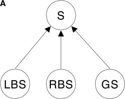
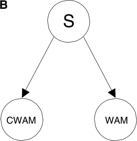
Bayesian networks (Pearl 1998) are graphical representations of probabilistic dependencies among evidence and variables of interest. Several applications of this frame-work to molecular biology are described in Salzberg et al. (1998). To combine comparative features with traditional compositional evidence, we propose two Bayesian network models, a naive Bayesian network and a full Bayesian network. Both models are depicted in Figure 2. The naive Bayesian network integrates different pieces of evidence that are assumed to be independent of each other. Consider, for instance, the case of a comparative feature, CWAM, and a traditional compositional feature, WAM as shown in Figure 2. By naive Bayesian network, Pr(CW AM, W AM| S) = Pr(CW AM|S)Pr(W AM| S). A full Bayesian network, on the other hand, models the case in which the evidence is correlated. If such evidence were LBS and RBS, and GS, the probability Pr(LBS, RBS, GS| S) cannot be factored into simpler terms.
Figure 2.
Integration of various features is done using either A full Bayes network model or B naive Bayes. LBS, RBS, and GS denote three pieces of evidence and S denotes the states in the genomic sequence. The evidence could be either comparative or traditional genomic evidence, represented by predictions made by GENSCAN. The genomic states include exons, introns, or intergenic regions. The distribution defined by the full Bayesian model is Pr(LBS,RBS,GS| S) and allows no further factorization, whereas the naive Bayes allows decomposition Pr(CWAM,WAM| S) = Pr(CWAM| S)Pr(WAM| S).
As an initial test of whether and how the comparative evidence helps the compositional model identify the splice sites, we simplify the correlation between WAM and CWAM by assuming that they are independent and use the naive Bayesian network to integrate them together:
 |
1 |
Here, {xi-l,...,xi,...,xi + k} is a window of k + l + 1 nucleotides around position i in the human sequence—xi is the nucleotide at position i. Similarly, {Yi-l,...,Yi,...,Yi + k} is the window of HCIS around the same position. Si takes on values such as Si ε {donor site, not a donor site}. Each PCW AM(·| ·, k)and PW AM(·| ·, k) are, as described in earlier sections, columns of their corresponding CWAM and WAM matrices.
The full Bayesian network is used to combine comparative scores in coding and noncoding regions with GENSCAN predictions:
 |
LBSi and RBSi are, as before, the comparative scores at position i in the sequence. GENSCAN's prediction, GS, is taken to be either 0 (noncoding) or 1 (coding). Si denotes one of the possible coding or noncoding regions i, Si = {initial exon, internal exon at reading frame 0, intron at reading frame 0,...}.
In both cases, probabilities that characterize various dependencies can be obtained from data using maximum-likelihood estimation. The combined probabilities are then integrated with a model of a genomic sequence.
Model of Genomic Sequence Structure
The genomic sequence structure is modeled with a generalized Hidden Markov Model (Rabiner 1989; Burge and Karlin 1997). In this context, the work is similar to TWINSCAN (Korf et al. 2001) and GENOMESCAN (Yeh et al. 2001) that include explicit duration models of exons. The main difference is the number of comparative features we incorporated in the model as well as a substantial capability to incorporate additional evidence using Bayesian Network principles.
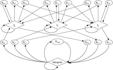
The model is shown in Figure 3. For simplicity, promoters, UTRs, poly(A), and the complementary strand are not accounted for in our model. In other genomic structures (exons, introns, etc.), comparative and traditional genomic scores were integrated using one of the above Bayesian methods. For instance, when LBS, RBS, and GENSCAN (GS) predictions are used, an exon in frame one of length N between positions i and i + N -1 is scored as: 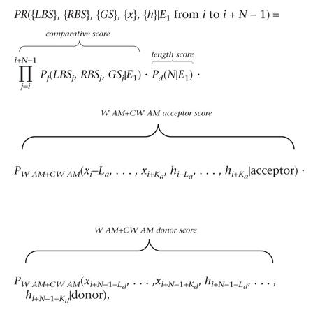 with {·} denoting the sequences of proposed features or DNA bases. Similar scoring methods are used for other functional elements, with the exception of introns, whose length distribution is exponential, and the score is simply, for instance, Pf(LBSi, RBSi, GSi| I1 at position i). Other combinations of comparative and genomic features were scored in the same fashion.
Figure 3.
Generalized Hidden Markov Model of genomic sequence structure. Each oval or diamond represents a unit in the genomic sequence as follows: intergenic; El,k, k = 0,1,2, three states for initial exons; ET,k, k = 0,1,2, three states for terminal exons; Esngl, single exon genes; El,k, l = 0,1,2 k = 0,1,2, internal exons at reading frames l; Il,l = 0,1,2, introns at reading frames l. Splice signals (donor and acceptor) and translational initiation and termination signals are subcomponents of exons and are not shown in the model. Promoters, 5′ and 3′ UTRs, poly(A) signals, and the complementary strand are not modeled. The length distribution of each coding state is modeled explicitly.
Evolutionary Analysis of Comparative Gene Prediction
Here, we address the problem of how the performance of a comparative gene finder depends on the evolutionary distance between the target and the reference organism. An answer to this problem may help one select the best pair of organisms for comparative genomic analysis and improve the quality of annotation. We were able recently to show (V. Pavlovic, L. Zhang, and S. Kasif, in prep.) (in a simplified setting) an exact formal relationship between the performance of a comparative gene finder and the evolutionary distance between genomes. Furthermore, we showed that there exists a distance in which the performance reaches a maximum. Similar conclusions are drawn in this work from a simulation study using synthetic human-reference homologs and a complex comparative gene finder. Moreover, our results here suggest that a mouse may not, on average, be the optimal reference for comparative analysis of the human genome.
Performance of any gene finder depends primarily on several key factors, including the distinctive signatures of different genomic regions. Because many of the top gene finders use probabilistic models to characterize genomic regions, one reasonable predictor of how well the gene finder will perform is the distance between the coding and noncoding probability distributions. One natural way to measure this distance is the relative entropy or Kullback-Liebler divergence7. We recently showed (V. Pavlovic, L. Zhang, and S. Kasif, in prep.) formally that the KL divergence, and, hence, the performance of a comparative gene finder, depends on evolutionary distance between genomic sequences used for comparative analysis.
To analyze how gene-finding performance depends on evolutionary distance, we consider a simplified model of a genomic sequence with only two regions, noncoding and coding. We assume that each region is homogeneous and is characterized by its own substitution rate matrix Q (Nei 2000). The substitution rate matrix could describe the substitution of bases (4 * 4 matrix) (Jukes and Cantor 1969; Kimura 1980), amino acids (20 * 20 matrix) (Jones et al. 1992), or codons (64 * 64 matrix) (Goldman and Yang 1994; Yang 1996]. For simplicity (Krogh et al. 1994), we assume that the noncoding and coding regions are characterized by base substitution matrices, Qn and Qc, respectively. Markov models of genomic evolution relate this rate to the probability of base substitution in the two regions:
 |
2 |
 |
3 |
with, for instance, Pc(t) = [Pc(i| j, t)]4 × 4 a probability substitution matrix whose entries are Pc(i| j, t) = Pr(base j substituted by base i at evolutionary time t).
In V. Pavlovic, L. Zhang, and S. Kasif (in prep.) we show that the gene-finding performance reaches a peak at some specific evolutionary distance, suggesting the pair of genomic sequences are best suited for comparative analysis. For the simplified gene-finding model, we can estimate the evolutionary distance exactly.
We characterized the substitutions in each of the coding and noncoding regions with a Jukes-Cantor (J-C) substitution model and computed the KL-divergence as a function of the evolutionary time, t.
Performance-Distance Analysis By Simulation
The explicit analysis of performance may be infeasible for most comparative gene-finding systems. As an alternative, we propose a simulation method to analyze the performance-distance correlation with a real comparative gene-prediction system. For each human sequence in our data set, we synthesize an orthologous sequence at different times t using an established evolutionary model. A comparative gene finder is then evaluated on each pair of human-synthetic orthologs and its performance is recorded.
Taking into account the preferred synonymous substitution and transition of the coding sequence through evolution, the coding regions are characterized by Yang's codon substitution model (64 * 64 matrix) (Yang et al. 2000). Yang's codon substitution model explicitly characterizes the synonymous/nonsynonymous ratios and transition/transversion ratios. Evolution in the noncoding regions is still characterized by a J-C substitution model (4 * 4 matrix). Given an alignment of two genomic sequences, a number of methods can be used to estimate the corresponding substitution probabilities, and in turn, the substitution rates (Nei 2000). Parameters in these two models were estimated on the human/mouse ortholog data set using the PAML (Phylogenetic analysis by maximum likelihood) package (Yang 1997). PAML outputs parameters that completely define substitution matrices, Qn and Qc, for both noncoding and coding regions. Synthetic orthologs were generated at different evolutionary times t = {t1 = 0,..., ti = 1,...,20} by sampling from the models in equations (2) and (3). The evolutionary time of ti = 1 corresponds to the distance between human and mouse8.
RESULTS AND DISCUSSION
Analysis of Comparative Features
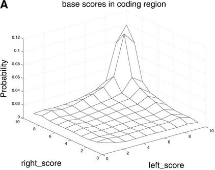
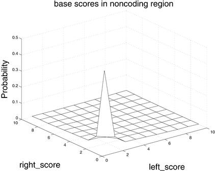
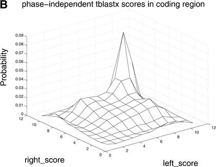
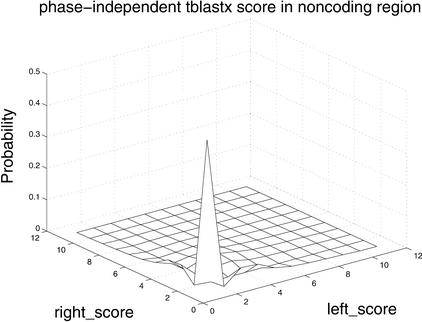
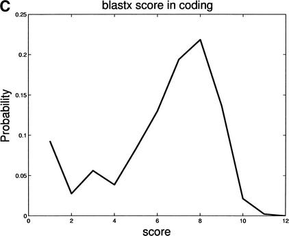
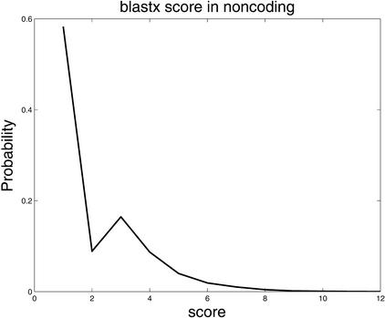
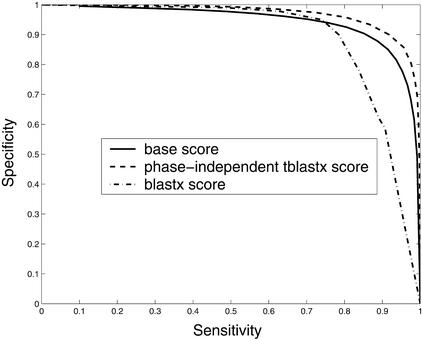
The distribution of comparative scores, displayed in Figure 4, shows that all three comparative scores, as expected, tend to be high in coding regions and low in noncoding regions. Furthermore, results of a more subtle analysis of their predictive capacity using the ROC method, shown in Figure 5, confirm the utility of these features. In Figure 5, phase-independent TBLASTX scores, with a precision of 0.97 are superior to the base scores (0.93) and the BLASTX scores (0.89). Although not shown, the ROC curve of the phase-dependent TBLASTX scores is very similar to that of its phase-independent counterpart.
Figure 4.
Differences in distributions of comparative scores in coding and noncoding regions indicate their potential utility. Shown are (A) distributions of RBS and LBS Pr(RBS,LBS| coding) and Pr(RBS,LBS| noncoding); (B) distributions of phase-independent TBLASTX scores; and (C) distributions of BLASTX scores.
Figure 5.
ROC analysis of ability of the base scores, phase-independent TBLASTX scores, and BLASTX scores to identify protein-encoding regions. Average accuracies of methods that use these scores are base scores, 0.93; phase-independent TBLASTX scores, 0.97; BLASTX scores, 0.89.
Difference in performance between the base scores and the TBLASTX scores is primarily due to the amino-acid nature of TBLASTX scores—TBLASTX scores measure similarity on amino acid level, whereas the base scores compare DNA sequences. Although most coding regions remain conserved on the DNA level, conservation also occurs extensively in noncoding sequences. However, in the conserved noncoding regions, similarity of translated amino acid sequences may not be significant because of different selective restrictions. On the other hand, although the conservation on DNA level is only moderate in synonymous substitution-rich coding regions, the amino acid conservations stay high. Therefore, TBLASTX scores have more significant correlation to coding regions than the base scores. The performance of phase-dependent TBLASTX scores is not noticeably better than that of phase-independent, because the window length (60–100 nucleotides) is short, and only in few cases can an out-of-phase TBLASTX bitscore be greater than the in-phase one. In other words, in most cases, the phase-independent TBLASTX scores is just the in-phase phase-dependent TBLASTX score. We also observed a relatively inferior performance of the BLASTX scores. One possible explanation is that strong BLASTX scores tend to be internal to exons and fail to accurately identify exonic boundaries. Windowed versions of BLASTX scores, such as those used in GENOMESCAN (Yeh et al. 2001), are therefore helpful in improving the performance.
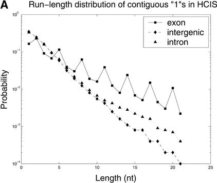
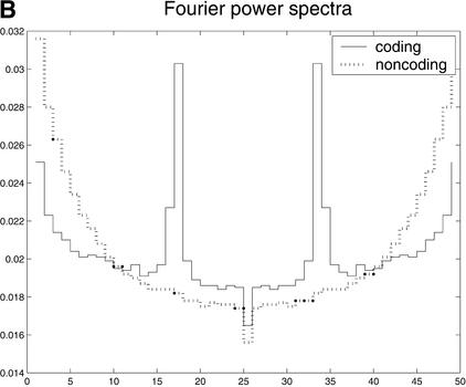
Additional results of HCIS analysis, depicted in Figure 6, emphasize one important feature in coding sequences, the preferred synonymous substitutions at the third codon position. A prime example of this is the result of the run-length analysis, shown in Figure 6A. In noncoding regions (both intergenic and intronic), the run-length distributions are geometric, implying a random distribution of substitutions/gaps. However, in coding regions, the length distribution peaks at each 3n + 2, n = 0, 1,.... This implies preferred occurrence of 0s, or mismatch/gap, at every third position. The second feature, a Fourier analysis of HCIS is shown in Figure 6B. Strong peaks in the Fourier power spectrum of the coding sequence correspond to a period of 3, confirming again a preferred occurrence of 0s. Thus, both the run-length distribution and Fourier analysis provide a good characterization of different selective pressures (enrichment of synonymous substitutions) in coding and noncoding sequences. However, our analysis also shows that, at present, the HCIS scores are weaker indicators than the comparative scores. A number of causes may explain this performance; although synonymous substitution-rich regions tend to be coding, coding regions can be strongly conserved, allowing few substitutions. Moreover, whereas most synonymous substitutions occur at the third codon position, not all third position substitutions are synonymous. This immediately suggests that one may be able to use some estimates of synonymous/nonsynonymous substitution ratios as scoring features. Unfortunately, these estimates rely heavily on the knowledge of base pair phases in both homologous sequences, a piece of information unavailable to this type of comparative gene finder. If one were to use a different gene-finder structure that maintains information about both phases, such as that of a product HMM (XHMM) (Walker et al. 2002), the synonymous/nonsynonymous ratio could be added as another comparative feature.
Figure 6.
(A) The run-length distributions of continuous 1s in HCIS in exon, intron, and intergenic sequences. (B) Fourier power spectrum of HCIS at coding (solid line) and noncoding (broken-dot line) regions. The peak corresponding to zero frequency has been omitted.
Comparative Analysis of Splice Sites and Translational Initiation/Termination Sites
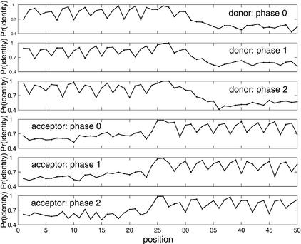
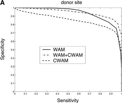
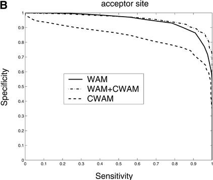
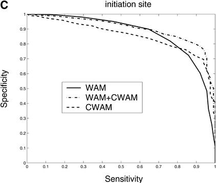
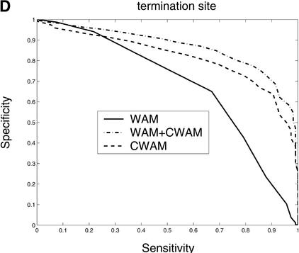
Consensus genomic sequences that signal the start and termination of translation and boundaries between exons and introns are known to represent good descriptors of translational initiation/termination sites and splice sites. Our comparative analysis shows that there is a significant change of similarity at the coding/noncoding junctions, and each kind of site displays a characteristic comparative consensus pattern as in Figure 7. This, in turn, implies that reasonable models of these comparative consensus patterns (for example, our CWAM model) may be useful in identifying such sites. Results of ROC analysis, shown in Figure 8, confirm this conjecture. Figure 8 illustrates the ROC performance of WAM, CWAM, and WAM + CWAM models for detecting donor, acceptor, translational initiation, and termination sites. As individual detectors of donor, acceptor, and translational initiation sites, CWAM models reveal performance inferior to the WAM. However, combined CWAM + WAM models achieved significantly better performance than traditional WAM models. More importantly, for detecting translational termination sites, CWAM alone outperformed the WAM, whereas the combined WAM + CWAM model remains superior to both simpler models. The improved performance of WAM + CWAM over WAM clearly implies that the detection of comparative features positively complements the traditional compositional models. The improved performance of the combined model, CWAM + WAM, also confirmed that the Bayesian network provides a reasonable model to combine different pieces of evidence together.
Figure 7.
Conservative patterns at the splice sites of introns in different phases. The Pr(identity) on y-axis stands for probability of identity at each position on the alignment. Positions 26 and 27 in the donor site correspond to GT, the terminal residues of the intron at the 5′ splice site, and positions 25 and 26 in the acceptor site correspond to AG, the terminal residues of the intron at the 3′ splice site. It can be seen that exonic regions not only are more conserved than intronic regions, but also display phase-dependent conservative patterns, which agree well with the preferred substitution in the third codon positions in the coding regions.
Figure 8.
Comparison of the performance of CWAM, WAM, and WAM + CWAM models on detecting the splice sites and translational initiation and termination sites with an ROC analysis. The performance is evaluated by leave-one-out cross-validation, i.e., the model is trained on all but one sequence and then evaluated on the remaining sequence. Performance is finally averaged over all such possible partitions. (A) Donor site, the area under each ROC curve is WAM, 0.93; CWAM, 0.85; WAM + CWAM, 0.94. (B) Acceptor site, the area under each ROC curve is WAM, 0.95; CWAM, 0.84; WAM + CWAM, 0.96. (C) Translational initiation site, the area under each ROC curve is WAM, 0.87; CWAM, 0.85; WAM + CWAM, 0.90. (D) Translational termination site, the area under each ROC curve is WAM, 0.68; CWAM, 0.82; WAM + CWAM, 0.86.
Comparative Human Gene Prediction
First, we investigate the ability of each comparative feature alone as the detector of protein-coding regions within a gene-prediction system. Then, we analyze whether these comparative features can complement a compositional gene finder (e.g., GENSCAN) by using the prediction of GENSCAN as additional evidence and integrating it with the comparative evidence. The prediction performance is evaluated on the 97 sequences in Batzoglou's data set by leave-one-out cross-validation, as summarized in Table 1. With only comparative evidence, the phase-independent TBLASTX scores yielded performance superior to other comparative features. Although this follows the conclusions of the independent ROC analysis, it should be noted that the performance achieved with only comparative evidence significantly lags behind the predictive abilities of GENSCAN. In general, gene-identification performance with comparative evidence alone is inferior to GENSCAN, showing lower sensitivity and specificity measured on both the base and the exon levels. This can be explained by the simplicity of comparative features as well as the integrator and genomic structure models that do not utilize positional dependency of comparative scores.
Table 1.
Prediction Performance With Different Pieces of Evidence
| Number of exons | Correct exons | Approx. exons | bSN | bSP | eSN | eSP | ME | WE | |
|---|---|---|---|---|---|---|---|---|---|
| AN | 386 | ||||||||
| GS | 417 | 272 | 286 | 0.96 | 0.91 | 0.63 | 0.61 | 0.03 | 0.08 |
| AS | 838 | 95 | 137 | 0.87 | 0.66 | 0.17 | 0.10 | 0.04 | 0.47 |
| TS | 375 | 58 | 72 | 0.92 | 0.75 | 0.19 | 0.18 | 0.09 | 0.17 |
| BS | 185 | 32 | 42 | 0.45 | 0.68 | 0.16 | 0.18 | 0.51 | 0.34 |
| GS + AS | 446 | 284 | 311 | 0.98 | 0.92 | 0.71 | 0.66 | 0.02 | 0.12 |
| GS + TS | 413 | 282 | 306 | 0.98 | 0.94 | 0.70 | 0.68 | 0.03 | 0.08 |
| GS + TPS | 417 | 278 | 304 | 0.98 | 0.94 | 0.70 | 0.67 | 0.03 | 0.10 |
| GS + BS | 429 | 278 | 304 | 0.98 | 0.92 | 0.69 | 0.66 | 0.03 | 0.11 |
| GS + TS + BS | 415 | 281 | 306 | 0.98 | 0.95 | 0.70 | 0.68 | 0.03 | 0.08 |
Performance comparison of gene identification with GS(GENSCAN), AS (base score), TS (phase-independent TBLASTX score), BS (BLASTX score), GS + AS (GENSCAN and base score), GS + TS (GENSCAN and phase-independent TBLASTX score), GS + TPS (GENSCAN and phase-dependent TBLASTX score), GS + BS (GENSCAN and BLASTX score), and GS + TS + BS (GENSCAN and phase-independent TBLASTX score and BLASTX score). The performance is evaluated by leave-one-out cross-validation. The model is trained on all but one sequence and then evaluated on the remaining sequence. Performance is finally averaged over all such possible partitions. (AN) Annotation. (Correct exons) Predicted exons whose both boundaries are correctly predicted. (Approx exons) Predicted exons with both boundaries close to the boundaries of annotated exons (<10 nts). (bSN) base sensitivity, (bSP) base specificity, (eSN) exon sensitivity, (eSP) exon specificity, (ME) missing exons, and (WE) wrong exons are estimated following Burset and Guigo (1996).
By combining comparative evidence with GENSCAN predictions, we achieved a noticeable improvement over the original GENSCAN performance. Both the sensitivity and specificity, as well as the number of correctly predicted exons, increased by including the comparative features. On the other hand, the combination of GENSCAN, phase-independent TBLASTX scores, and BLASTX scores (GS + TS + BS) did not lead to noticeably improved performance over the combination of GENSCAN and the phase-independent TBLASTX scores (GS + TS). Detailed study implies that careful selection of genomic features is needed and blind inclusion of additional noisy and contradicting features can sometimes lead to inferior performance. Our results confirmed that the comparative evidence could complement the GENSCAN by using the simple binary predictions (coding/noncoding) of GENSCAN. Improved performance may be expected by an alternative utilization of GENSCAN results. For instance, the exon probability might be more informative than the coding/noncoding predictions.
We also compare our system (GS + TS) with TWINSCAN (Korf et al. 2001), SLAM (Pachter et al. 2002), as well as GENSCAN (Burge and Karlin 1997) on SGP2 data set (Parra et al. 2003), which contains both single-gene sequences (IMOG data set) and multi-gene sequences (BI data set). Our system is trained on the 97 sequences in Batzoglou's data set (sequences that are homologous to the testing sequences have been removed out of the training data set). As summarized in Table 2, our system outperforms others on the IMOG data set. However, the performance is inferior to that of the other systems on the BI data set. Detailed study reveals that BI data set contains genes on the complementary strand, which our current model does not account for.
Table 2.
Evaluation of Prediction Performance
| Number of exons IMOG/BI | Correct exons IMOG/BI | Approx. exons IMOG/BI | bSN IMOG/BI | bSP IMOG/BI | eSN IMOG/BI | eSP IMOG/BI | ME IMOG/BI | WE IMOG/BI | |
|---|---|---|---|---|---|---|---|---|---|
| AN | 70/86 | ||||||||
| GS + TS | 71/102 | 61/34 | 62/60 | 0.97/0.95 | 0.98/0.84 | 0.85/0.38 | 0.84/0.30 | 0.03/0.07 | 0.05/0.20 |
| GS | 68/92 | 59/42 | 60/75 | 0.97/0.97 | 0.94/0.69 | 0.71/0.46 | 0.74/0.30 | 0.03/0.04 | 0.04/0.25 |
| TWS | 49/79 | 31/36 | 34/57 | 0.79/0.73 | 0.85/0.82 | 0.62/0.40 | 0.63/0.37 | 0.25/0.31 | 0.04/0.19 |
| SLM | 63/77 | 52/35 | 55/69 | 0.89/0.88 | 0.97/0.87 | 0.81/0.39 | 0.82/0.36 | 0.08/0.10 | 0.01/0.11 |
Comparison of our prediction system (GS + TS) with GENSCAN (GS), TWINSCAN (TWS), and SLAM (SLM) on the IMOG and BI data set of SGP2 data set. Performance is estimated on each sequence and averaged over all sequences in the corresponding data set.
It is noted that whereas we used a global alignment (GLASS) in our system, global alignments will not, in general, be able to account for duplications and inversions in the genome. We believe that, in general, both local and global alignments should be experimented with and applied as appropriate. In fact, our full system is based on a combination of both local and global alignments. First, long orthologous regions are identified using local alignment strategies (e.g., BLAST). Then, these orthologous regions are aligned by either local or global alignment, depending on which might give the better results, to show the conservative features in different genomic regions. We believe that a proper combination of local and global alignments may generate the best results. For instance, local alignment usually induces significant hits around the centers of exonic regions, whereas the alignment in the exon boundaries tends to be poor. Nevertheless, our study shows that the comparative features at the exon boundaries can significantly enhance the identification of splice sites.
Evolutionary Analysis of Comparative Gene Prediction
Evolutionary analysis of comparative gene finding, outlined above, reveals two important results.
We show that, using a simplified gene-finding model, the performance of comparative gene analysis depends on evolutionary distance between genomes and conservation properties of different genomic regions. Furthermore, there exists a distance in which the performance reaches a maximum.
Simulation study using synthetic human-reference homologs and a complex comparative gene finder reaffirms the performance-distance dependency suggested by the simple model. Moreover, it reveals that mouse may not, on average, be the optimal reference for comparative analysis of the human genome.
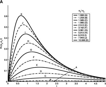
To qualitatively illustrate how gene-finding performance depends on evolutionary distance, we first consider a simplified model of a genomic sequence described in the Methods section. Both regions are homogeneous and are characterized by J-C (Jukes and Cantor 1969) substitution models. Each substitution matrix Q in the J-C model is characterized by a parameter α; conservation rates (main diagonal of Q) are -3α, whereas all substitution rates (all other entries of Q) are α. We have assumed that noncoding and coding regions are, therefore, characterized by parameters αn and αc, respectively. Using the methodology presented in V. Pavlovic, L. Zhang, and S. Kasif (in prep.) and in the simplified model, we show that KL divergence and, hence, the error and the precision9 of annotation now become a relatively simple function of the evolutionary distance t. This is depicted in Figure 9A. Optimal divergence times t*, for which the KL divergence (precision) is maximized and the error is minimized, vary with differences in the substitution models of the two regions. As expected, larger differences in base substitution models (signified by the ratio αc/αn) cause shorter optimal divergence times t*. Moreover, the shorter optimal times are also related to higher values of the maximal KL divergence, implying smaller errors. Hence, if the two regions show significant differences in conservation rates, the optimal pairs of species need to be less diverged, and consequently, the error in comparative genomic prediction is expected to decrease.
Figure 9.
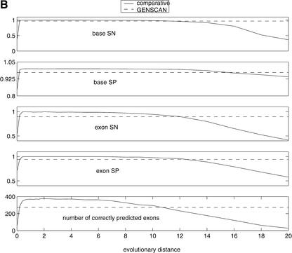
(A) Precision (KL-divergence in the figure) as a function of divergence time. Through evolution, coding and noncoding regions are characterized with Jukes-Cantor substitution models with parameters αc and αn, respectively. We set αc = 0.1and the ratio of αn/αc is sampled from 1–10. Larger differences between parameters imply shorter optimal time t* required for minimal prediction error. Similarly, the more different the conservation rates of the two regions are, the higher the precision is. (B) Performance of human gene prediction was evaluated on synthetic orthologs at different evolutionary distances. The evolutionary distance of 1 corresponds to the distance between human and mouse. In all cases, comparative gene finder outperforms GENSCAN (indicated by broken lines) on the plateau between the distances of 0.5 and 6. Performance degrades significantly for very low and very high distances.
The J-C model represents one of the simplest models of molecular evolution. For example, it does not account for the existence of conserved noncoding regions that was confirmed recently by cross-species comparison of orthologous sequences (Wasserman and Fickett 1998; Levy et al. 2001; Waterston et al. 2002). The functions of these regions are typically unknown and cannot be explained by classical evolutionary models. Nevertheless, for an initial analysis of the performance versus divergence relationship, the J-C model yields a first-of-a-kind analytical answer, as well as a fair characterization of a majority of coding and noncoding regions (homogeneous assumption). As a follow-up to our initial analysis, more realistic and complex models are possible. For instance, each region (coding or noncoding) can be described as having several subregions with different rates, similar to heterogeneous models of Yang (1996) and Yang and Nielsen (2002).
Explicit formal analysis of performance may be infeasible for most comparative gene finders. As an alternative, we used a simulation method to access the same performance-distance trends with a real gene-prediction system. For each target sequence in the data set, we synthesize an orthologous reference sequence at different times t. A comparative gene finder can then be evaluated on each pair of human-synthetic orthologs and its performance recorded.
Our simulation study revealed a correlation of performance and evolutionary distance (Fig. 9B). Similar to the simple model, the performance of the complex gene finder degraded at very low (<1) and very high (>6) evolutionary distances. Unlike the KL-divergence analysis, the analysis on simulated orthologs displayed a wider plateau of good performance, above GENSCAN alone, covering a region of distances from 0.5–6. This may be a consequence of a number of factors that play roles in the complex comparative gene finder but are absent from the simple computational model. For instance, the real gene prediction is generated by Viterbi decoding and is a complex function of the splice sites, the gene structure model, the frame consistency, and many other factors, as well as the evolutionary time. Another interesting result is revealed by the simulation analysis. Although mouse (at evolutionary distance 1) lies in the plateau region, results also indicate that improved performance may occur with a genome at about twice the evolutionary distance of the mouse (distance 1.8 in Fig. 9B). For instance, the data set of orthologs at distance 1.8 displays a total of 359recovered exons, whereas in the original human–mouse data set, only 323 exons are correctly predicted. This result reaffirms the need for careful selection of genomic sequences at evolutionary distances appropriate for comparative analysis. With the rapid pace of sequencing of orthologous sequences in different species, a similar test on real sequences is becoming possible and will be discussed in a separate study.
Summary
Novel gene discovery in large eukaryotic genomes remains a significant scientific challenge. Recent comparison of the Celera and Ensembl-predicted human gene sets reveals that nearly 80% of the novel transcripts were predicted by one of the annotation teams and not the other (Hogenesch et al. 2001). Furthermore, the exact number of human genes and their precise locations vary dramatically with different prediction systems (Crollius et al. 2000; Ewing and Green 2000; Liang et al. 2000). The sequencing of model genomes provides an unprecedented opportunity to analyze gene structures in the human genome from a comparative perspective, and possibly substantially improve the quality of human genome annotation. Consequently, several pioneering systems have been developed to identify human genes using the mouse genome as reference (Batzoglou et al. 2000; Korf et al. 2001; Yeh et al. 2001; Meyer and Durbin 2002; Pachter et al. 2002; Parra et al. 2003).
The first question addressed in this work is whether the mouse provides an ideal reference for human gene identification. Our preliminary simulation study provides a positive answer. We proposed a simplified computational model to explicitly represent the performance of gene prediction as a function of evolutionary distance. The evolutionary analysis predicts the existence of an evolutionary distance that provides an optimal accuracy in comparative gene prediction. To investigate the correlation of evolutionary time and gene prediction accuracy with a realistic gene finder, we used synthetic sequences as the reference for human gene prediction. Synthetic sequences over a wide range of evolutionary distances are shown to deliver reasonable performance. Although the mouse sequence falls in the high-accuracy range, better performance is predicted at an evolutionary distance beyond that of human and mouse.
The second question we address is what comparative features can most improve the accuracy of gene prediction. Our analysis of the exon boundaries shows a characteristic comparative pattern at each of the donor, acceptor, translational initiation, and termination sites. A first-order comparative Markov model (CWAM) is proposed to characterize these comparative patterns. ROC and other analyses confirm that these comparative features positively complement more frequently used compositional models. Additionally, a variety of comparative features are introduced and studied in terms of their potential to distinguish coding from noncoding sequences. Our results (using both ROC analysis and comparative gene prediction) suggest that local TBLASTX scores, which measure the conservation of translated amino acid sequences, perform best for identifying the protein-coding regions.
Finally, we investigated the integration of different sources of evidence for effective gene prediction. We experimented with a simple Bayesian network combiner that complements a GENSCAN style generalized HMM gene model. The resulting architecture combines comparative evidence, predictions made by GENSCAN, comparative and compositional models of splice sites, translational initiation/termination sites, and a variety of other features. Compared with TWINSCAN, SLAM, and GENSCAN, our system shows comparable or better performance. Our results suggest that Bayesian networks provide a flexible and convenient methodology for evidence integration.
Acknowledgments
We thank the anonymous referees for their very useful comments and suggestions. L.Z. thanks Dr. Joel Graber for helpful discussions. L.Z. was supported by Sequenom Inc. V.P. and S.K. were supported by NSF (KDI).
The publication costs of this article were defrayed in part by payment of page charges. This article must therefore be hereby marked “advertisement” in accordance with 18 USC section 1734 solely to indicate this fact.
[Software is available on request from the authors.]
Article and publication are at http://www.genome.org/cgi/doi/10.1101/gr.703903. Article published online before print in May 2003.
Footnotes
Although BLOSUM80 is expected to better characterize the divergence between human and mouse protein, we experimented with both BLOSUM62 and BLOSUM80 and found that BLOSUM62 was slightly better than, although very similar to, BLOSUM80 at identifying protein-coding regions. Hence, we used BLOSUM62 in our experiments. All other BLAST parameters are used as defaults.
 |
It can be shown that one type of annotation error depends on the KL divergence as error ∼ exp(-KL). See V. Pavlovic, L. Zhang, and S. Kasif(in prep.) for more details.
Stated more precisely, results of maximum likelihood estimation are not the substitution matrices Q themselves, but rather the estimates of products Q′ = Q · t′, in which t′ is the distance between human and mouse. Hence, substituting Q′ and t = 1 in, for instance, (2) yields the exponent Q′ · t = Q′ · 1 = Q · t′· 1 = Q · t′, and, thus, the probability of substitutions at the evolutionary distance between human and mouse.
Error = exp(-KL[Pc∥Pn]). Precision = 1 - error.
References
- Altschul, S.F., Madden, T.L., Schaffer, A.A., Zhang, J., Zhang, Z., Miller, W., and Lipman, D.J. 1997. Gapped blast and psi-blast: A new generation of protein database search programs. Nucleic Acids Res. 25: 3389–3402. [DOI] [PMC free article] [PubMed] [Google Scholar]
- Batzoglou, S., Pachter, L., Mesirov, J., Berger, B., and Lander, E. 2000. Human and mouse gene structure: Comparative analysis and application to exon prediction. Genome Res. 10: 950–958. [DOI] [PMC free article] [PubMed] [Google Scholar]
- Birney, E. and Durbin, R. 2000. Using GeneWise in the Drosophila annotation experiment. Genome Res. 10: 547–548. [DOI] [PMC free article] [PubMed] [Google Scholar]
- Burge, C. and Karlin, S. 1997. Prediction of complete gene structures in human genomic dna. J. Mol. Biol. 268: 78–94. [DOI] [PubMed] [Google Scholar]
- Burset, M. and Guigo, R. 1996. Evaluation of gene structure prediction programs. Genomics 34: 353–367. [DOI] [PubMed] [Google Scholar]
- Cai, D., Delcher, A., Kao, B., and Kasif, S. 2000. Modeling splice sites with bayes networks. Bioinformatics 16: 152–158. [DOI] [PubMed] [Google Scholar]
- Claverie, J. 1997. Computational methods for the identification of genes in vertebrate genomic sequences. Hum. Mol. Genet. 6: 1735–1744. [DOI] [PubMed] [Google Scholar]
- Claverie, J. 1998. Computational methods for exon detection. Mol. Biotechnol. 10: 27–48. [DOI] [PubMed] [Google Scholar]
- Cover, T. and Thomas, J. 1991. Elements of information theory. John Wiley and Sons, New York, NY.
- Crollius, H.R., Jaillon, O., Bernot, A., Dasilva, C., Bouneau, L., Fischer, C., Fizames, C., Wincker, P., Brottier, P., Qutier, F., et al. 2000. Estimate of human gene number provided by genome-wide analysis using Tetraodon nigroviridis DNA sequence. Nat. Genet. 25: 235–238. [DOI] [PubMed] [Google Scholar]
- Egan, J. 1975. Signal detection theory and ROC analysis. Academic Press, New York, NY.
- Ewing, B. and Green, P. 2000. Analysis of expressed sequence tags indicates 35,000 human genes. Nat. Genet. 25: 232–234. [DOI] [PubMed] [Google Scholar]
- Fickett, J. 1996. The gene identification problem: An overview for developers. Comput. Chem. 20: 103–118. [DOI] [PubMed] [Google Scholar]
- Gelfand, M.S., Mironov, A.A., and Pevzner, P.A. 1996. Gene recognition via spliced sequence alignment. Proc. Natl. Acad. Sci. 93: 9061–9066. [DOI] [PMC free article] [PubMed] [Google Scholar]
- Goldman, N. and Yang, Z. 1994. A codon-based model of nucleotide substitution for protein-coding DNA sequences. Mol. Biol. Evol. 11: 725–736. [DOI] [PubMed] [Google Scholar]
- Hogenesch, J., Ching, K., Batalov, S., Su, A., Walker, J., Zhou, Y., Kay, S., Schultz, P., and Cooke, M. 2001. A comparison of the Celera and Ensembl predicted gene sets reveals little overlap in novel genes. Cell 106: 413–415. [DOI] [PubMed] [Google Scholar]
- Hubbard, T., Barker, D., Birney, E., Cameron, G., Chen, Y., Clark, L., Cox, T., Cuff, J., Curwen, V., Down, T., et al. 2002. The Ensembl genome database project. Nucleic Acids Res. 30: 38–41. [DOI] [PMC free article] [PubMed] [Google Scholar]
- Jones, D.T., Taylor, W.R., and Thornton, M. 1992. The rapid generation of mutation data matrices from protein sequences. Comput. Appl. Biosci. 8: 275–282. [DOI] [PubMed] [Google Scholar]
- Jukes, T.H. and Cantor, C.R. 1969. Evolution of protein molecules. In Mammalian protein metabolism III. (ed. H.N. Munro), pp. 21–132. Academic Press, New York, NY.
- Kimura, M. 1980. A simple method for estimating evolutionary rates of base substitutions through comparative studies of nucleotide sequences. J. Mol. Evol. 16: 111–120. [DOI] [PubMed] [Google Scholar]
- Korf, I., Flicek, P., Duan, D., and Brent, M. 2001. Integrating genomic homology into gene structure prediction. Bioinformatics 17: S140–S148. [DOI] [PubMed] [Google Scholar]
- Krogh, A. 1997. Two methods for improving performance of an HMM and their application for gene finding. In Proceedings of Fifth International Conference on intelligent systems for molecular biology, pp. 179–186. AAAI Press, Menlo Park, CA. [PubMed]
- Krogh, A., Mian, I.S., and Haussler, D. 1994. A hidden Markov model that finds genes in E. coli DNA. Nucleic Acids Res. 22: 4768–4778. [DOI] [PMC free article] [PubMed] [Google Scholar]
- Kulp, D., Haussler, D., Reese, M.G., and Eeckman, F.H. 1996. A generalized Hidden Markov Model for the recognition of human genes in DNA. Intell. Syst. Mol. Biol. AAAI/MIT Press, St. Louis, MO. [PubMed]
- Lander, E., Linton, L.M., Birren, B., Nusbaum, C., Zody, M.C., Baldwin, J., Devon, K., Dewar, K., Doyle, M., Fitzhugh, W., et al. 2001. Initial sequencing and analysis of the human genome. Nature 409: 860–921. [DOI] [PubMed] [Google Scholar]
- Levy, S., Hannenhalli, S., and Workman, C. 2001. Enrichment of regulatory signals in conserved non-coding genomic sequence. Bioinformatics 17: 871–877. [DOI] [PubMed] [Google Scholar]
- Liang, F., Holt, I., Pertea, G., Karamycheva, S., Salzberg, S.L., and Quackenbush, J. 2000. Gene index analysis of the human genome estimates approximately 120,000 genes. Nat. Genet. 25: 239–240. [DOI] [PubMed] [Google Scholar]
- Meyer, I. and Durbin, R. 2002. Comparative ab initio prediction of gene structures using pair hmms. Bioinformatics 18: 1309–1318. [DOI] [PubMed] [Google Scholar]
- Mural, R., Adams, M.D., Myers, E.W., Smith, H.O., Miklos, G.L., Wides, R., Halpern, A., Li, P.W., Sutton, G.G., Nadeau, J., et al. 2002. A comparison of whole-genome shotgun-derived mouse chromosome 16 and the human genome. Science 296: 1661–1671. [DOI] [PubMed] [Google Scholar]
- Nei, M. and Kumar, S. 2000. Molecular evolution and phylogenetics. Oxford University Press, New York.
- Pachter, L., Alexandersson, M., and Cawley, S. 2002. Applications of generalized pair hidden markov models to alignment and gene finding problems. J. Computat. Biol. 9: 389–400. [DOI] [PubMed] [Google Scholar]
- Parra, G., Blanco, E., and Guigo, R. 2000. GeneID in Drosophila. Genome Res. 10: 511–515. [DOI] [PMC free article] [PubMed] [Google Scholar]
- Parra, G., Agarwal, P., Abril, J., Wiehe, T., Fickett, J., and Guig, R. 2003. Comparative gene prediction in human and mouse. Genome Res. 13: 108–117. (data set available at http://www1.imim.es/datasets/humanmouse/). [DOI] [PMC free article] [PubMed]
- Pavlovic, V., Garg, A., and Kasif, S. 2002. A bayesian framework for combining gene predictions. Bioinformatics 18: 19–27. [DOI] [PubMed] [Google Scholar]
- Pearl, J. 1998. Probability reasoning in intelligence system. Morgan Kaufmann, San Mateo, CA.
- Rabiner, L.R. 1989. A tutorial on hidden markov models and selected applications in speech recognition. Proceedings of the IEEE 77: 257–286. [Google Scholar]
- Rogic, S., Mackworth, A., and Ouellette, F. 2001. Evaluation of gene-finding programs on mammalian sequences. Genome Res. 11: 817–832. [DOI] [PMC free article] [PubMed] [Google Scholar]
- Salzberg, S.L. 1997. A method for identifying splice sites and translational start sites in eukaryotic mRNA. Comput. Appl. Biosci. (CABIOS) 13: 365–376. [DOI] [PubMed] [Google Scholar]
- Salzberg, S., Searls, D., and Kasif, S. 1998. Computational methods in molecular biology. In New comprehensive biochemistry, Vol. 32. Elsevier Science B.V., Amsterdam, Netherlands.
- Venter, J., Adams, M.D., Meyers, E.W., Li, P.W., Mural, R.J., Sutton, G.G., Smith, H.O., Yandell, M., Evans, C.A., Holt, R.A., et al. 2001. The sequence of the human genome. Science 291: 1304–1351. [DOI] [PubMed] [Google Scholar]
- Walker, M., Pavlovic, V., and Kasif, S. 2002. A comparative genomic method for computational identification of prokaryotic translation initiation sites. Nucleic Acids Res. 30: 3181–3191. [DOI] [PMC free article] [PubMed] [Google Scholar]
- Wasserman, W. and Fickett, J. 1998. Identification of regulatory regions which confer muscle-specific gene expression. J. Mol. Biol. 278: 167–181. [DOI] [PubMed] [Google Scholar]
- Waterston, R.H., Lindblad-Toh, K., Birney, E., Rogers, J., Abril, J.F., Agarwal, P., Agarwala, R., Arinscough, R., Alexandersson, M., An, P., et al 2002. Initial sequencing and comparative analysis of the mouse genome. Nature 420: 520–562. [DOI] [PubMed] [Google Scholar]
- Yang, Z. 1996. Maximum-likelihood models for combined analyses of multiple sequence data. J. Mol. Evol. 42: 587–596. [DOI] [PubMed] [Google Scholar]
- Yang, Z. 1997. Paml: A program package for phylogenetic analysis by maximum likelihood. Comp. Appl. Biosci. 13: 555–556. [DOI] [PubMed] [Google Scholar]
- Yang, Z. and Nielsen, R. 2002. Codon-substitution models for detecting molecular adaptation at individual sites along specific lineages. Mol. Biol. Evol. 19: 908–917. [DOI] [PubMed] [Google Scholar]
- Yang, Z., Nielsen, R., Goldman, N., and Pedersen, A. 2000. Codon-substitution models for heterogeneous selection pressure at amino acid sites. Genetics 155: 431–449. [DOI] [PMC free article] [PubMed] [Google Scholar]
- Yeh, R., Lim, L., and Burge, C. 2001. Computational inference of homologous gene structures in the human genome. Genome Res. 11: 803–816. [DOI] [PMC free article] [PubMed] [Google Scholar]
- Zhang, M. 1997. Identification of protein coding regions in the human genome by quadratic discriminant analysis. Proc. Natl. Acad. Sci. 94: 565–568. [DOI] [PMC free article] [PubMed] [Google Scholar]
- Zhang, M. 2002. Computational prediction of eukaryotic protein-coding genes. Nat. Rev. Genet. 3: 698–709. [DOI] [PubMed] [Google Scholar]
WEB SITE REFERENCES
- http://linkage.rockefeller.edu/wli/gene/; Web site for the bibliograph on computational gene recognition.
- http://www.cbc.umn.edu/ResearchProjects/BIBLIOGRAPHY/gene_finding/gene_finding.html; Web site for the bibliograph on computational gene recognition.


