Structure-based analysis of single nucleotide variants in the renin-angiotensinogen complex

Abstract

The Renin-Angiotensin System (RAS) plays an important role in regulating blood pressure and controlling sodium levels in the blood. Hyperactivity of this system has been linked to numerous conditions including hypertension, kidney disease, and congestive heart failure. As such, various classes of drugs have been developed to inhibit this system. These drugs are aimed at preventing angiotensin II from performing its function by inhibiting angiotensin II receptors or inhibiting angiotensin-converting enzyme from converting angiotensin I to angiotensin II. The last class of inhibitors is aimed at preventing angiotensin I from being formed by preventing renin from interacting with a plasma protein called angiotensinogen. In this study, we provide a structure-based analysis of the effect of single nucleotide variants on the interaction between renin and angiotensinogen with the aim of revealing important residues and potentially damaging variants.

Introduction

The Renin-Angiotensin System (RAS) is responsible for the regulation of blood pressure and sodium homeostasis [1]. This is achieved by producing angiotensin II, a potent, 8-residue vasoconstrictor, which causes the arterioles to constrict, resulting in increased blood pressure. Angiotensin II also stimulates the release of aldosterone, which increases the rate at which sodium ions are reabsorbed into the blood [2].

When RAS is activated, the juxtaglomerular cells in the kidneys secrete renin into the blood. Once in the blood, renin cleaves angiotensin I, a 10-residue peptide, from a plasma protein known as angiotensinogen, which originates in the liver. Angiotensin I is then converted to angiotensin II by angiotensin-converting enzyme (ACE), which cleaves a further two residues from the former [2].

Hyperactivity of RAS has been linked to high blood pressure (hypertension), congestive heart failure, and kidney disease. As such, various classes of drugs have been developed to inhibit this system including ACE inhibitors [3], Angiotensin Receptor Blockers (ARBs) [4], and renin inhibitors [5].

In this study, we have used structural bioinformatics and network analysis techniques to investigate the effect of non-synonymous Single Nucleotide Variants (SNVs) on renin-angiotensinogen interaction to identify important residues and potentially damaging SNVs.

Material and methods

Data retrieval

Sequences and suitable Protein Data Bank (PDB) [6] structures for renin and angiotensinogen were identified via a search of the – Human Mutation Analysis (HUMA) [7] database. The amino acid sequences were then downloaded from Uniprot. Structures were evaluated for suitability based on their coverage of the target sequences and their PDB validation metrics, before being downloaded from the PDB. All available SNVs for each protein were then downloaded from HUMA.

Homology modeling – wild type

To account for missing residues in existing experimental structures, the renin-angiotensinogen complex was modeled using MODELLER [8]. The complex has been solved in 2X0B, which was used as the main template. Renin was covered by chain A of 2X0B. Three additional templates, 2WXY, 2WXW, and 2WXZ were used to cover gaps in chain B i.e. angiotensinogen. Alignment of the templates to the target sequences was performed using PROMALS3D [9].

After aligning, the first 73 residues of the renin target sequence, and the first 32 residues and last 3 residues of the angiotensinogen target sequence, were not covered by the templates. These residues were trimmed from the alignment as a result. One hundred models were then generated using ‘very slow’ refinement.

Model evaluation

One hundred models of the renin-angiotensinogen complex were generated. The top three models were then selected based on their DOPE Z-Score [10], and further evaluated using PROCHECK [11], VERIFY3D [12], and PROSA [13] to validate that they were indeed accurate models. The best model was then chosen based on the combination of these results.

SNV filtering

The SNV data set, obtained from HUMA, contains all SNVs from dbSNP [14] that could be mapped to the renin and angiotensinogen protein sequences based on their chromosome coordinates. As such, the resulting data set contained synonymous and nonsense SNVs. Synonymous SNVs result in no change in the amino acid sequence. They are, therefore, unlikely to have any structural effects on the protein, and were removed from the data set. Nonsense SNVs, on the other hand, result in early stop codons. These SNPSs are highly likely to be damaging as they usually result in non-functioning proteins. As such, there was little reason to further analyze these SNVs in this paper and they were also removed from the data set.

VAPOR [15], a workflow that combines the results of PolyPhen-2 [16], Provean [17], PhD-SNP [18], PANTHER-PSEP [19], and FATHMM [20] to predict the functional effect of SNVs, was then used to predict which of the remaining SNVs were likely to cause conformational changes that would alter the functionality of the protein. If more than one program predicted that the SNV was neutral, we removed it from the data set. One exception to this is if there was a known disease-association in the HUMA database.

Lastly, we used the Protein Interactions Calculator (PIC) [21] to determine which residues in the complex were interacting. The final data set contained all SNVs that were at the interface between the two proteins and were either predicted to be damaging or were interacting with a position at which a SNV occurred in the other protein.

Homology modeling – mutants

The SNVs identified in the previous step were introduced into the structures via homology modeling. Models were generated for each SNV individually. Additional models were then generated where SNVs occurred at the interacting positions in both renin and angiotensinogen. In these cases, the mutants were introduced to both protein sequences in the complex before being modeled. This resulted in a combination of models that accounted for each SNV occurring on its own as well as SNVs that might co-occur with SNVs in interacting positions – potentially compensating SNVs.

The same modeling methodology was used as for the wild type. 2X0B, 2WXY, 2WXW, and 2WXZ, were once again used as templates. Alignment was performed using PROMALS3D and 100 models were generated for each modeling run. The best model for each mutant and mutant combination was then picked based on DOPE Z-Scores. As these models were very similar to the wild type, it was not deemed necessary to repeat the other evaluation methods to confirm the quality.

Molecular Dynamics

Homology models produced in the previous steps were free from any non-standard residues or missing atoms and were thus ready for Molecular Dynamics (MD) simulations. The simulations were performed for each of the complexes using GROMACS 5.1 [22] on 480 CPU cores at the Centre for High Performance Computing (CHPC) in Cape Town, South Africa. The all-atom AMBER03 force field was employed for topology generation and energy calculations. Simple point charge water was added for solvation, after which the system was neutralized using 0.15M NaCl in a triclinic periodic box with a clearance space of 1.5 angstroms from the protein. The system was then relaxed by energy minimization using the method of steepest descent with a force tolerance of 1000kJ/mol/nm capped at an upper limit of 50,000 steps. Short range cut-offs (Van der Waals and Coulombic interactions) were set at 1nm each, while long-distance electrostatics were handled by the Particle-mesh Ewald algorithm [23]. Temperature was equilibrated at 310K over a period of 100ps, using the modified Berendsen thermostat [24]. Pressure equilibration ensued, using the Parrinello-Rahman barostat [25] to maintain the pressure at 1bar. Production dynamics were finally run over 100ns periods with 2fs time steps, writing coordinates every 5000 steps. The LINCS algorithm [26] was applied to correct for rotational bond lengthening during the MD runs.

Analysis of MD trajectories

Preliminary Root Mean Square Deviation (RMSD) analysis revealed jumps that occurred in several complexes despite our first attempts to correct for periodic boundary conditions using molecular center of mass. Trajectories were thus sequentially corrected for periodic boundary conditions by first making the proteins whole, followed by the removal of jumps across boundaries and finally centering the protein inside the simulation box. RMSD was computed from Cα atoms after least square fitting along the respective protein backbones. Additionally, Root Mean Square Fluctuation (RMSF) calculations were evaluated to monitor residue motion (averaged over residue atoms) across the entire production run.

Dynamic Network Analysis (evaluation at SNV locations)

In order to calculate the Residue Interaction Network (RIN) over each production MD frame, multi-PDB files were first generated using GROMACS tool for trajectory conversion. An in-house Python script was then designed to predict residue interaction by evaluating pairwise residue distances between all Cβ (or Cα in the case of glycine) atoms for each complex, looped across all frames. A cut-off distance of 6.7 angstroms [27] was used to define any residue-residue contact (contact = 1, no contact = 0) around designated SNV positions. A total of 10,001 frames (in PDB format) were traversed to generate edge lists that were used by an in-house R script – using the igraph library [28] – to produce a weighted adjacency matrix, which was converted to frequencies by dividing by the number of frames, similar to the approach used by Doshi et al [29]. Edge weights were displayed as log2 re-scaled values, while the contact frequencies were used as edge labels. The weighted RINs of the wild type proteins were compared to their mutant counterparts at analogous positions to assess gain or loss of contact.

Dynamic Network Analysis (ΔL)

The shortest path (L_ij) between two nodes, i and j, in a network is equal to the minimum number of edges that must be traversed to reach j from i. The average shortest path (L_i) to a node, i, is the average of all the shortest paths to i from all other nodes in the network. Given a RIN, where each node is a residue in a protein structure, Dijkstra’s shortest path algorithm [30] can be used to produce an N x N matrix of all-vs-all shortest path lengths, where N is the number of residues in the protein. Getting the mean of each column in this matrix results in an N x 1 matrix, where each value corresponds to the average shortest path length to the respective residue.

For every MD run, an implementation of Dijkstra’s shortest path algorithm in the NetworkX Python library [31], in conjunction with the NumPy python library [32], was used in a custom Python script to calculate the average path matrices for RINs at 10ns intervals (including the RIN at time = 0). As such, for each 100ns MD run, 11 average shortest path matrices were calculated. The mean and standard deviation of these matrices were then calculated.

The mean of the matrices represents the average L of each of the residues over the 100ns run, while the standard deviation represents how much L of each residue fluctuates over the 100ns. The values were plotted to an ‘Average L vs Residue Number’ graph using Matplotlib [33]. In addition to calculating L, ΔL/L was calculated for all residues after each 10ns interval by getting the difference between the L at time = 0 and L at the respective time point and normalizing by dividing by the original L. The mean and standard deviation of ΔL/L over the 100ns were calculated in the same way as described above and plotted using Matplotlib.

Dynamic Network Analysis (ΔBC)

Given a node, i, betweenness centrality (BC_i) is a measurement of how often shortest paths in a network run through i. As such, it is a measure of how central a node is for efficient navigation of the network. BC can be calculated using Ulrik Brandes algorithm [34].

For each MD run, an implementation of Ulrik Brandes algorithm in the NetworkX library was used to compute BC for all RINs at 1ns intervals (including the RIN at time = 0). This resulted in 101 N x 1 matrices. As with ΔL/L above, ΔBC was calculated by finding the difference between the BC at each time point and BC at time = 0 (BC values were already normalized using the NetworkX library function). The mean ΔBC and standard deviation of ΔBC for each residue were then calculated as described ΔL/L.

Results and Discussion

Homology modeling – wild type

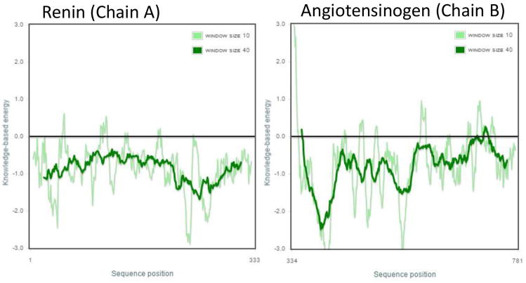
Homology models of the renin-angiotensinogen complex were generated using MODELLER. All models produced were evaluated using DOPE Z-Scores, PROCHECK, PROSA, and VERIFY3D. The top model of the complex had a DOPE Z-Score of −1.20, while PROCHECK calculated that 90.2% of residues were in most favored regions, and VERIFY3D calculated that 80.8% of residues had a 3D-1D score >= 0.2. PROSA results were also positive and are depicted in Figure 1.

Figure 1.

PROSA results for the renin-angiotensinogen complex.

SNV filtering

All 317 SNVs for renin and 212 SNVs for angiotensinogen were downloaded from HUMA. Synonymous and nonsense SNVs were removed from the data set. The remaining 130 renin SNVs and 198 angiotensinogen SNVs were submitted to VAPOR for functional predictions. For angiotensinogen, VAPOR produced results from PolyPhen-2, Provean, PhD-SNP, FATHMM, and PANTHER-PSEP (S-Data 1). If more than one of these tools predicted that an SNV would not have a deleterious effect, the SNV was removed from the data set. The only exception to this was if the SNV was associated with a disease in the HUMA database. In this case, it was retained. The same process was followed with renin (S-Data 2). In renin’s case, PANTHER-PSEP was unable to produce results. The resulting data set held 85 damaging angiotensinogen SNVs and 39 damaging renin SNVs.

We further filtered this data set by only focusing on residues at the interface between renin and angiotensinogen. All damaging SNVs in the interface were retained in the data set. In addition, if a renin SNV was found to be interacting with an SNV in angiotensinogen, both were retained, regardless of the VAPOR predictions. The final data set contained 9 angiotensinogen SNVs (Table 1) and 6 renin SNVs (Table 2).

Table 1.

SNV data set for angiotensinogen

dbSNP ID	Residue Change	Location	Reason for inclusion
rs539231427	H39R	Interface	Highly damaging prediction by VAPOR Interacts with position in renin where SNV occurs
rs746613821	P40L	Interface	Highly damaging prediction by VAPOR Interacts with position in renin where SNV occurs
rs41271499	L43F	Interface	Highly damaging prediction by VAPOR Interacts with position in renin where SNV occurs
rs760531325	E48K	Interface	Interacts with position in renin where SNV occurs
rs751752211	S49G	Interface	Interacts with position in renin where SNV occurs
rs377047370	S49N	Interface	Highly damaging prediction by VAPOR Interacts with position in renin where SNV occurs
rs201406560	A104T	Interface	Interacts with position in renin where SNV occurs
rs767370325	M105V	Interface	Interacts with position in renin where SNV occurs
rs756744141	D168Y	Interface	Highly damaging prediction by VAPOR Interacts with position in renin where SNV occurs

Table 2.

SNV data set for renin

dbSNP ID	Residue Change	Location	Reason for inclusion
rs868694193	D104N	Interface	Highly damaging prediction by VAPOR Interacts with position in angiotensinogen where SNV occurs
rs191049685	R148C	Interface	Interacts with position in angiotensinogen where SNV occurs
rs371704012	R148H	Interface	Interacts with position in angiotensinogen whre SNV occurs
rs770190833	A188V	Interface	Highly damaging prediction by VAPOR
rs752426689	L318R	Interface	Interacts with position in angiotensinogen where SNV occurs
rs201922371	F319V	Interface	Interacts with position in angiotensinogen where SNV occurs

Homology modeling – mutants

In total, 25 mutant models of the renin-angiotensinogen complex were produced (Table 3). Models were named based on the SNV that they contained and the chain that the SNV occurred in. For example, in model “ang_P40L”, an SNV occurs at position 40 in angiotensinogen (chain B) and results in a substitution of Proline for Leucine. Similarly, in “ren_A188V”, an SNV occurs at position 188 in renin (chain A) and results in a substitution of Alanine for Valine.

Table 3.

Mutant models of the renin-angiotensinogen complex

Model	DOPE Z-Score	Renin (chain A) mutants	Angiotensinogen(chain B) mutants
ren_D104N	−1.20	rs868694193
ren_R148C	−1.19	rs191049685
ren_R148H	−1.20	rs371704012
ren_A188V	−1.19	rs770190833
ren_L318R	−1.18	rs752426689
ren_F319V	−1.17	rs201922371
ang_H39R	−1.18		rs539231427
ang_P40L	−1.18		rs746613821
ang_L43F	−1.18		rs41271499
ang_E48K	−1.18		rs760531325
ang_S49G	−1.21		rs751752211
ang_S49N	−1.21		rs377047370
ang_A104T	−1.20		rs201406560
ang_M105V	−1.18		rs767370325
ang_D168Y	−1.19		rs756744141
ren_D104N_ang_L43F	−1.20	rs868694193	rs41271499
ren_R148C_ang_E48K	−1.17	rs191049685	rs760531325
ren_R148C_ang_S49G	−1.19	rs191049685	rs751752211
ren_R148C_ang_S49N	−1.20	rs191049685	rs377047370
ren_R148H_ang_E48K	−1.18	rs371704012	rs760531325
ren_R148H_ang_S49G	−1.20	rs371704012	rs751752211
ren_R148H_ang_S49N	−1.20	rs371704012	rs377047370
ren_L318R_ang_A104T	−1.20	rs752426689	rs201406560
ren_F319V_ang_A104T	−1.19	rs201922371	rs201406560
ren_F319V_ang_M105V	−1.20	rs201922371	rs767370325

In addition to introducing SNVs into a structure individually, mutant models were produced with combinations of SNVs. If an SNV occurred at a position in renin that interacts with a position in angiotensinogen where another SNV occurred, a model was produced containing both of these potentially compensating SNVs. For example, model “ren_D104N_ang_L43F” contains and SNV at position 104 in renin and position 43 in angiotensinogen and, in the wild type, these positions were calculated to be interacting.

Molecular Dynamics

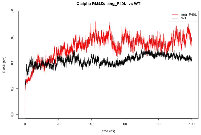
The wild type complex and the 25 mutant complexes were subjected to 100ns MD simulations. Of the 26 simulations, 25 completed successfully. Only ren_L318R failed due to a bad contact with water. Due to already having a large amount of data and the fact that L318R in renin was not predicted to be damaging by VAPOR, we decided not to resolve this. Of the 25 successful simulations (S-Data 3), only ang_P40L had still not stabilized after the full 100ns (Figure 2). The SNV, P40L, occurs in the loop region of angiotensinogen, which is cleaved by renin to become angiotensin 1. As such, the instability may indicate that this SNV plays an important role in the binding of renin to angiotensinogen.

Figure 2.

RMSD of the complex containing the SNV, P40L, in angiotensinogen. This is the only mutation tested that destabilizes the complex.

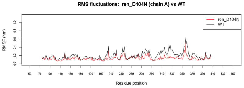
RMSF was calculated for all successful MD runs (S-Data 4). The overall trend across mutant complexes revealed an increase in rigidity compared to the wild type, especially in the region from residue 260 to 380 in renin. This increased rigidity was noticeable in the complex containing the renin SNV, D104N (Figure 3), which, according to HUMA, is associated with Renal Tubular Dysgenesis.

Figure 3.

RMSF of ren_D104V. Increased rigidity is noticeable from residue 260 to 380 of renin (chain A) in disease-associated model, ren_D104V.

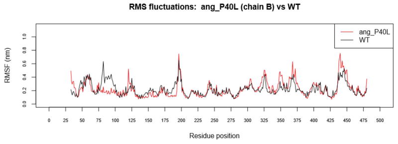
The difference in rigidity is less pronounced in other complexes, however, such as ang_P40L (Figure 4). While ang_P40L was not be able to stabilize over 100ns, it seems that most of the fluctuation occurs in the angiotensinogen side of the complex. In angiotensinogen, ang_P40L has increased RMSF between residues 300 to 380. Only ren_A188V and ren_R148C_ang_E48K show signs of similar fluctuation in this region.

Figure 4.

RMSF ang_P40L. Increased fluctuation is noticeable in ang_P40L between residue 300 and 380 of angiotensinogen (chain B).

Almost all mutations resulted in increased rigidity from residue 75 to 100 in angiotensinogen. Additionally, increased rigidity was noticeable between residue 175 and 200 in angiotensinogen. The latter region is located on the inside of the former, while also being near to the interface of the two proteins. It is possible that mutations occurring in the interface help to hold this region steady, which in turn holds the region containing residues 75 to 100 steady.

A spike in the RMSF was seen between residue 435 and 450 in a number of the mutant models. This is a loop region far from the interface and, as such, high flexibility is not surprising here, nor is it likely to be damaging.

Network Analysis

Changes in the RINs of the models were measured by calculating the average and standard deviation of ΔBC (S-Data 5) and ΔL/L (S-Data 6) for each MD simulation. The standard deviation provided a measurement of how much BC and L fluctuated over the course of the run, while the average values provided an idea of what regions experienced a more permanent increase or decrease in BC and L. Additionally, residue contact maps were calculated for the positions where the SNVs occurred (S-Data 7).

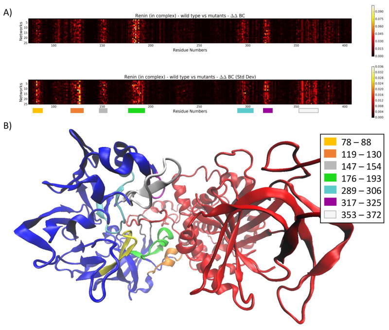
In terms of BC, mutations produced a fairly consistent pattern of changes to the network when compared to the wild type. In renin, significant changes could be seen in 7 regions, depicted in Figure 5. Interestingly, mutations resulted in significant changes to the network in regions far from where the SNV was located. Additionally, affected regions were centered around the interface between the proteins. This is not surprising, as the interface is a high traffic zone for network communication and, as such, mutations which shift these areas slightly could have a significant impact on inter-protein communication.

Figure 5.

A) A heat map depicting the absolute difference between ΔBC in the wild type (first row) and ΔBC in the mutants (ΔΔBC) in chain A (renin) of the complex. Most differences are confined to the color-coded regions. B) The renin-angiotensinogen complex. The areas consisting of large changes in BC in renin (red) have been mapped to the structure.

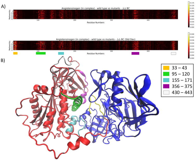
Mutations have a similar effect on angiotensinogen. Changes in BC are most notable in 5 regions (Figure 6). While 4 of these regions were located at the complex interface, the region consisting of residues 430 to 443 (white) did not contain any interacting residues.

Figure 6.

A) A heat map depicting the absolute difference between ΔBC in the wild type (first row) and ΔBC in the mutants (ΔΔBC) in chain B (angiotensinogen) of the complex. B) The areas consisting of large changes in BC in angiotensinogen (blue) have been mapped to the complex structure.

Regions in the complex revealed by the analysis of ΔBC may depict areas that reorganize to compensate for mutations. Such reorganization would be important for the protein to retain its function when mutations occur.

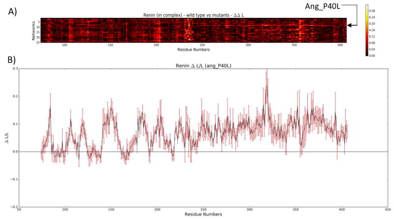
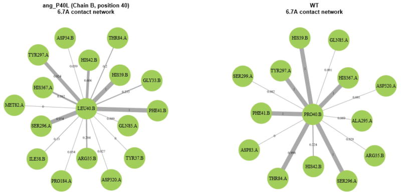
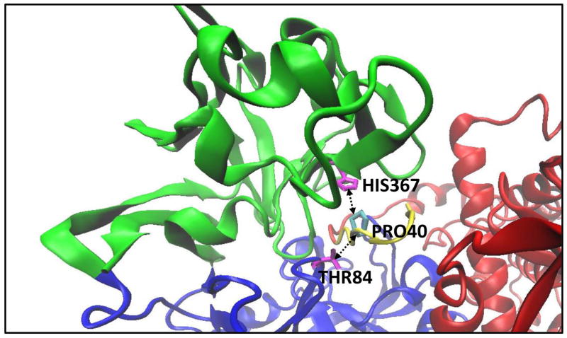
When analyzing ΔL/L, two mutants, in particular, caught the eye. The first was ang_P40L. The average ΔL/L for ang_P40L was high across most of the second half of the renin sequence (from approximately residue 245 until the end of the sequence), as can be seen in Figure 7. Looking at the contact network for residue 40 of angiotensinogen (Figure 8), we can see that two prominent contacts in the wild type (PRO40.B-THR84.A and PRO40.B-HIS367.A) that are maintained consistently throughout the simulation of the wild type (99.8% and 100% of the time, respectively) are reduced to occasional contacts in the mutant (20% and 39.2% of the time, respectively). Upon further examination of the structure (Figure 9), we see that THR84.A and HIS367.A are important residues for providing access to the part of the structure with increased ΔL/L. As such, it can be seen that the loss of these contacts results in decreased accessibility to the back half of renin – an increased ΔL/L means that the average path to these residues is increased. Further work is required to determine whether this loss in accessibility would result in negative effects, such as a reduced ability of renin to cleave angiotensin 1 from angiotensinogen.

Figure 7.

A) Heat map representing the absolute difference in ΔL/L between the wild type renin and the mutants. The mutant complex, ang_P40L, stands out from residue 245 until the end of renin. B) Closer inspection of ang_P40L shows an elevated ΔL/L for the later part of renin, while the standard deviation, depicted by the red error bars, remains relatively small.

Figure 8.

Residue contact map of ang_P40L (left) and the wild type (right) complexes. Interaction with HIS367.A and THR84.A is severely reduced in the mutant complex.

Figure 9.

Interface of renin-angiotensinogen wild type. Residues HIS367 and THR84 in renin interact with PRO40 in angiotensinogen. In ang_P40L, Proline is replaced with Leucine and the interaction is severely reduced. In addition, ΔL/L for the region corresponding to residue 245 to 407 (green). As such, it appears that the loss of these two interactions affects the accessibility of this region.

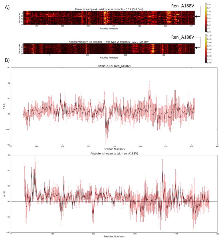
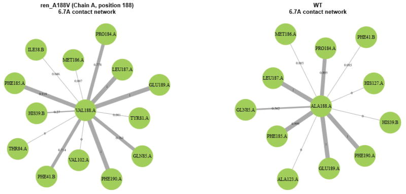
The second interesting mutant was ren_A188V. In contrast to ang_P40L, the average ΔL/L remained relatively constant across this complex. However, when looking at the standard deviation (Figure 10), it can be seen that the ΔL/L of ren_A188V fluctuated heavily across most of renin and parts of angiotensinogen. Looking at the residue contact map of ren_A188V (Figure 11), the VAL188.A interacts with PHE41.B more often than ALA188.A in the wild type (71.4% vs 8.5% respectively). As PHE41.B is in a loop region, which is likely flexible, interacting with this residue may cause the renin structure to shift more. That the contact happens 71.4% of the time in the mutant also means that the bond is being continuously broken and reformed, which could also explain the fluctuation.

Figure 10.

A) A heat map depicting the difference in the standard deviation of the average ΔL/L between wild type and the mutants. The mutant complex, ren_A188V, appears to fluctuate more than the other complexes. B) Large error bars in the ΔL/L plot indicate that ren_A188V fluctuated heavily over the 100ns MD simulation.

Figure 11.

The residue contact map for ang_A188V (left) and the wild type (right). The interaction between PHE41.B occurs more often in the mutant complex.

Conclusions

The Renin-Angiotensin System plays an important role in regulating arterial blood pressure and plasma sodium levels. To produce angiotensin 1, renin cleaves a 10-residue peptide from angiotensinogen. We have used structural bioinformatics and network analysis techniques to analyze the effects of SNVs at the interface between renin and angiotensinogen.

A total of 25 successful MD simulations were run to perform this analysis. Of the 25 MD runs, only the complex containing the SNV, P40L, in angiotensinogen did not stabilize after 100ns. After further analyzing this complex, it was found that this mutation resulted in a loss of interaction between position 40 in angiotensinogen and position 84 and 367 in renin. This resulted in a significant decrease in the accessibility of a large section of the renin structure. Additionally, it was found that the complex containing the SNV, A188V, in renin was subject to significant fluctuation in ΔL/L. This was potentially due to increased interaction between position 188 in renin and position 41 in angiotensinogen.

Based off of these results, we found that using network analysis techniques in combination with MD provided useful insights into the function of the protein complex. It was especially useful for finding important interacting residues, such as PRO40 in angiotensinogen and HIS367 and THR84 in renin. However, areas of high and low ΔBC and ΔL/L do not correlate directly with RMSF. This may be due to the fact that RMSF measures the movement of a residue, whereas network analysis techniques such as BC and L also take the movement of surrounding residues into account. In other words, a change in the BC and L of a residue does not necessarily mean that that residue is, itself, moving. It might be that the residues around it are moving, affecting shortest paths that usually traverse it. As such, network analysis should be used in conjunction with RMSF to fully understand the movement of a protein or protein complex.

Abbreviations

ACE

Angiotensin Converting Enzyme

ARB

Angiotensin Receptor Blocker

BC

Betweenness Centrality

L

Average shortest path

MD

Molecular Dynamics

RAS

Renin-Angiotensinogen System

RIN

Residue Interaction Network

RMSD

Root Mean Square Deviation

RMSF

Root Mean Square Fluctuation

SNV

Single Nucleotide Variant

References

- 1.Kobori H, Nangaku M, Navar LG, Nishiyama A. The intrarenal renin-angiotensin system: from physiology to the pathobiology of hypertension and kidney disease. Pharmacol Rev. 2007;59:251–87. doi: 10.1124/pr.59.3.3. [DOI] [PubMed] [Google Scholar]
- 2.Paul M, Poyan MA, Kreutz R. Physiology of local renin-angiotensin systems. Physiol Rev. 2006;86:747–803. doi: 10.1152/physrev.00036.2005. [DOI] [PubMed] [Google Scholar]
- 3.Sweitzer NK. What Is an Angiotensin Converting Enzyme Inhibitor? Circulation. 2003;108:16–8. doi: 10.1161/01.CIR.0000075957.16003.07. [DOI] [PubMed] [Google Scholar]
- 4.Barreras A, Gurk-Turner C. Angiotensin II receptor blockers. Proc (Bayl Univ Med Cent) 2003;16:123–6. doi: 10.1080/08998280.2003.11927893. [DOI] [PMC free article] [PubMed] [Google Scholar]
- 5.Israili ZH. Renin inhibitors as antihypertensive agents. Rev Latinoam Hipertens. 2008;3:98–112. doi: 10.1097/MJT.0b013e3181c08096. [DOI] [Google Scholar]
- 6.Berman HM, Westbrook J, Feng Z, Gilliland G, Bhat TN, Weissig H, et al. The Protein Data Bank. Nucleic Acids Res. 2000;28:235–42. doi: 10.1093/nar/28.1.235. [DOI] [PMC free article] [PubMed] [Google Scholar]
- 7.HUMA. 2016 [Google Scholar]
- 8.Sali A, Blundell TL. Comparative protein modelling by satisfaction of spatial restraints. J Mol Biol. 1993;234:779–815. doi: 10.1006/jmbi.1993.1626. [DOI] [PubMed] [Google Scholar]
- 9.Pei J, Kim BH, Grishin NV. PROMALS3D: A tool for multiple protein sequence and structure alignments. Nucleic Acids Res. 2008;36:2295–300. doi: 10.1093/nar/gkn072. [DOI] [PMC free article] [PubMed] [Google Scholar]
- 10.Shen M-Y, Sali A. Statistical potential for assessment and prediction of protein structures. Protein Sci. 2006;15:2507–24. doi: 10.1110/ps.062416606. [DOI] [PMC free article] [PubMed] [Google Scholar]
- 11.Laskowski RA, MacArthur MW, Moss DS, Thornton JM. PROCHECK: a program to check the stereochemical quality of protein structures. J Appl Crystallogr. 1993;26:283–91. doi: 10.1107/S0021889892009944. [DOI] [Google Scholar]
- 12.Eisenberg D, Lüthy R, Bowie JU. VERIFY3D: Assessment of protein models with three-dimensional profiles. Methods Enzymol. 1997;277:396–406. doi: 10.1016/S0076-6879(97)77022-8. [DOI] [PubMed] [Google Scholar]
- 13.Wiederstein M, Sippl MJ. ProSA-web: Interactive web service for the recognition of errors in three-dimensional structures of proteins. Nucleic Acids Res. 2007:35. doi: 10.1093/nar/gkm290. [DOI] [PMC free article] [PubMed] [Google Scholar]
- 14.Sherry ST, Ward MH, Kholodov M, Baker J, Phan L, Smigielski EM, et al. dbSNP: the NCBI database of genetic variation. Nucleic Acids Res. 2001;29:308–11. doi: 10.1093/nar/29.1.308. [DOI] [PMC free article] [PubMed] [Google Scholar]
- 15.VAPOR. n.d https://huma.rubi.ru.ac.za/#vapor.
- 16.Adzhubei IA, Schmidt S, Peshkin L, Ramensky VE, Gerasimova A, Bork P, et al. A method and server for predicting damaging missense mutations. Nat Methods. 2010;7:248–9. doi: 10.1038/nmeth0410-248. [DOI] [PMC free article] [PubMed] [Google Scholar]
- 17.Choi Y, Sims GE, Murphy S, Miller JR, Chan AP. Predicting the Functional Effect of Amino Acid Substitutions and Indels. PLoS One. 2012:7. doi: 10.1371/journal.pone.0046688. [DOI] [PMC free article] [PubMed] [Google Scholar]
- 18.Capriotti E, Calabrese R, Casadio R. Predicting the insurgence of human genetic diseases associated to single point protein mutations with support vector machines and evolutionary information. Bioinformatics. 2006;22:2729–34. doi: 10.1093/bioinformatics/btl423. [DOI] [PubMed] [Google Scholar]
- 19.Tang H, Thomas PD. PANTHER-PSEP: predicting disease-causing genetic variants using position-specific evolutionary preservation. Bioinformatics. 2016:1–3. doi: 10.1093/bioinformatics/btw222. [DOI] [PubMed] [Google Scholar]
- 20.Shihab HA, Gough J, Cooper DN, Stenson PD, Barker GL, Edwards KJ, et al. Predicting the functional, molecular, and phenotypic consequences of amino acid substitutions using hidden Markov models. Hum Mutat. 2013;34:57–65. doi: 10.1002/humu.22225. [DOI] [PMC free article] [PubMed] [Google Scholar]
- 21.Tina KG, Bhadra R, Srinivasan N. PIC: Protein Interactions Calculator. Nucleic Acids Res. 2007:35. doi: 10.1093/nar/gkm423. [DOI] [PMC free article] [PubMed] [Google Scholar]
- 22.Abraham MJ, Murtola T, Schulz R, Páll S, Smith JC, Hess B, et al. GROMACS: High performance molecular simulations through multi-level parallelism from laptops to supercomputers. SoftwareX. 2015;1:19–25. doi: 10.1016/j.softx.2015.06.001. [DOI] [Google Scholar]
- 23.Darden T, York D, Pedersen L. Particle mesh Ewald: An N·log(N) method for Ewald sums in large systems. J Chem Phys. 1993;98:10089. doi: 10.1063/1.464397. [DOI] [Google Scholar]
- 24.Berendsen HJC, Postma JPM, van Gunsteren WF, DiNola a, Haak JR. Molecular dynamics with coupling to an external bath. J Chem Phys. 1984;81:3684–90. doi: 10.1063/1.448118. [DOI] [Google Scholar]
- 25.Parrinello M, Rahman A. Polymorphic transitions in single crystals: A new molecular dynamics method. J Appl Phys. 1981;52:7182–90. doi: 10.1063/1.328693. [DOI] [Google Scholar]
- 26.Hess B, Bekker H, Berendsen HJC, Fraaije JGEM. LINCS: A linear constraint solver for molecular simulations. J Comput Chem. 1997;18:1463–72. doi: 10.1002/(SICI)1096-987X(199709)18:12<1463::AID-JCC4>3.0.CO;2-H. [DOI] [Google Scholar]
- 27.Ozbaykal G, Rana Atilgan A, Atilgan C. In silico mutational studies of Hsp70 disclose sites with distinct functional attributes. Proteins Struct Funct Bioinforma. 2015;83:2077–90. doi: 10.1002/prot.24925. [DOI] [PubMed] [Google Scholar]
- 28.Csárdi G, Nepusz T. The igraph software package for complex network research. InterJournal Complex Syst. 2006:1695. [Google Scholar]
- 29.Doshi U, Holliday MJ, Eisenmesser EZ, Hamelberg D. Dynamical network of residue–residue contacts reveals coupled allosteric effects in recognition, catalysis, and mutation. Proc Natl Acad Sci. 2016;113:4735–40. doi: 10.1073/pnas.1523573113. [DOI] [PMC free article] [PubMed] [Google Scholar]
- 30.Dijkstra EW. A note on two problems in connexion with graphs. Numer Math. 1959;1:269–71. doi: 10.1007/BF01386390. [DOI] [Google Scholar]
- 31.Overview - NetworkX. 2016 https://networkx.github.io.
- 32.NumPy. 2016 n.d http://www.numpy.org/
- 33.Matplotlib: Python plotting. n.d http://matplotlib.org/
- 34.Brandes U. A faster algorithm for betweenness centrality*. J Math Sociol. 2001;25:163–77. doi: 10.1080/0022250X.2001.9990249. [DOI] [Google Scholar]
Associated Data
This section collects any data citations, data availability statements, or supplementary materials included in this article.