TOWARD BAYESIAN INFERENCE OF THE SPATIAL DISTRIBUTION OF PROTEINS FROM THREE-CUBE FÖRSTER RESONANCE ENERGY TRANSFER DATA

Abstract

Förster resonance energy transfer (FRET) is a quantum-physical phenomenon where energy may be transferred from one molecule to a neighbor molecule if the molecules are close enough. Using fluorophore molecule marking of proteins in a cell, it is possible to measure in microscopic images to what extent FRET takes place between the fluorophores. This provides indirect information of the spatial distribution of the proteins. Questions of particular interest are whether (and if so to which extent) proteins of possibly different types interact or whether they appear independently of each other. In this paper we propose a new likelihood-based approach to statistical inference for FRET microscopic data. The likelihood function is obtained from a detailed modeling of the FRET data-generating mechanism conditional on a protein configuration. We next follow a Bayesian approach and introduce a spatial point process prior model for the protein configurations depending on hyperparameters quantifying the intensity of the point process. Posterior distributions are evaluated using Markov chain Monte Carlo. We propose to infer microscope-related parameters in an initial step from reference data without interaction between the proteins. The new methodology is applied to simulated and real datasets.

1. Introduction

In the biology community there is a vast interest in studying the biomolecular structure and dynamics of macromolecular assemblies in order to understand their functions [Alber et al. (2017), Polo and Jackson (2011), Krissinel and Henrick (2007), Puglisi (2005)]. Because the interactions between proteins and the typical size of proteins (1–100 nm) is at the nanoscale level [Erickson (2009)], no information can be obtained from conventional optical microscopic techniques, which at best can resolve distances down to ~200 nm [van Putten et al. (2011)]. Instead, Förster resonance energy transfer—also referred to as fluorescence resonance energy transfer—microscopy is widely used to obtain such information. Förster resonance energy transfer (FRET) provides information about distances of the order of 2 to 10 nm within or between molecular structures and is the preferred tool for investigating spatial relationships in biochemistry [Wu and Brand (1994), Gryczynski, Gryczynski and Lakowicz (2005), Clegg (1995, 2006)].

FRET is the nonradiative transfer of the surplus of energy from an excited donor fluorophore (fluorescent molecule) to a sufficiently nearby acceptor fluorophore by dipole–dipole interaction [Heitler (1954), Rohatgi-Mukherjee (1978)]. The widespread use of FRET in biological research is based on the possibility to label, in vivo or in vitro, proteins with fluorophores that are spectrally matched [Miyawaki, Sawano and Kogure (2003), Bunt and Wouters (2004)]. The energy transfer due to the FRET mechanism is a stochastic process, and the probability that energy transfer occurs between a donor and an acceptor fluorophore is heavily dependent on the distance between them. The probability that energy transfer occurs is commonly referred to as the efficiency of the energy transfer. The usefulness of FRET lies in the fact that various techniques exist by which the fraction of donor excitations that result in energy transfer—that is, the efficiency—can be quantified.

Two main methods for determining the FRET efficiency are as follows: fluorescence lifetime measurements [Wallrabe and Periasamy (2005), Lakowicz (2009), Chen et al. (2013)] and spectral methods [Sun et al. (2011), Zimmermann, Rietdorf and Pepperkok (2003)]. We focus in this paper on the most commonly applied spectral method called three-cube FRET. Due to the FRET mechanism, a certain fraction of the de-excitations of a donor result in energy transfer to an acceptor instead of donor photon emission, thereby the rate by which photons are emitted from the donors decreases—a phenomenon referred to as quenching of the donor—while instead photons are emitted by the acceptors. Spectral methods now rely on determining the decrease in the donor emission due to FRET. For three-cube FRET, intensity measurements are carried out using three different filter sets—often referred to as cubes—each comprising an excitation filter, a dichroic mirror, and an emission filter. This results in three digital intensity images [Zal and Gascoigne (2004), Wallrabe et al. (2006), Periasamy et al. (2008), Periasamy and Day (2011)]. Two images are obtained by exposing the sample to light in the donor absorption spectrum and recording emitted intensities both in the donor and the acceptor excitation spectrum. The third image is obtained by exposing the sample to light in the acceptor spectrum and also recording light in the acceptor spectrum.

Given FRET image data, the task is to obtain information concerning the spatial configuration of the donors and acceptors in the sample. For example, Wallrabe et al. (2003) study the clustering of ligand–receptor complexes in endocytic membranes using confocal FRET microscopy. They differentiate between a clustered or a random distribution of proteins by considering the dependence of the FRET efficiency on donor and acceptor concentrations. In particular, independence of the efficiency on acceptor concentration or a decrease in the efficiency for a higher unquenched donor signal for a fixed acceptor concentration are both indicators for clustering [Kenworthy and Edidin (1998), Kenworthy (2001)]. Goswami et al. (2008) instead compare observed distributions of fluorescence intensity and fluorescence anisotropy with values expected from a Poisson distribution of nanoclusters.

Other, computational, approaches mainly rely on the construction of a configuration of donors and acceptors and computing the FRET efficiency related to this configuration by numerical computation of the energy transfer probabilities for each of the donors [Wolber and Hudson (1979), Corry, Jayatilaka and Rigby (2005)]. This simple approach has been extended by various authors by simulating FRET events explicitly using Monte Carlo techniques. The extended approach gives the possibility to include additional physical complexity into the model to account for possible photobleaching of donors and acceptors during a FRET measurement or the effect that temporarily unavailable acceptors can have on the FRET efficiency [Frederix et al. (2002), Berney and Danuser (2003), Corry, Jayatilaka and Rigby (2005)]. Corry, Jayatilaka and Rigby (2005) further carefully studied the FRET efficiency in relation to various fixed donor and acceptor configurations (e.g., pentamers) and give a concise overview of the development of the numerical Monte Carlo approaches.

Loura and Prieto (2011), Loura, Fernandes and Prieto (2010) and Lakowicz (2009) give excellent reviews of methods to extract spatial information in membrane biophysics from FRET data. Methods determining the complex structures of a protein or the spatial distribution of protein complexes in living cells are given in e.g. Raicu et al. (2009) and Bonomi et al. (2014).

The previous mentioned contributions are based on a detailed understanding of the FRET data generating mechanism. This knowledge, however, so far has not been applied to obtain a complete statistical model of FRET data allowing for a principled statistical analysis. In this paper we present a first attempt to conduct a full likelihood-based Bayesian analysis of three-cube FRET image data. The potential advantages of such an approach are that the posterior distribution gives detailed quantitative information regarding model parameters and donor–acceptor interactions as well as measures of uncertainty regarding this information. To obtain the likelihood function, we derive, based on physical considerations, an accurate statistical model for the distribution of the image intensities, conditional on a point pattern consisting of donors and acceptors. We further impose a spatial point process prior [Møller and Waagepetersen (2004)] for the unknown configuration of donors and acceptors. Since our resulting posterior distribution is of a complicated form, we use Markov chain Monte Carlo (MCMC) to sample from the posterior distribution [Gamerman and Lopes (2006), Gilks, Richardson and Spiegelhalter (1996)]. It is difficult to infer simultaneously microscope-related parameters and possible interactions between donors and acceptors. We therefore propose to infer microscope-related parameters in an initial step based on reference data without interactions between donors and acceptors. We asses the Bayesian inference procedure by a simulation study and by applying it to an empirical in-vitro reference dataset.

2. Observation model for three-cube FRET image data

A three-cube FRET dataset consists of three images each corresponding to a rectangular region W which is a union of rectangular pixels, W = ⋃_i∈𝒢C_i, indexed by a grid 𝒢. Each pixel C_i records a light intensity due to emission from donors or acceptors. The images are created by (1) excitation of donors and measurement of donor emission, (2) excitation of acceptors and measurement of acceptor emission or (3) excitation of donors and measurement of acceptor emission (due to FRET). We represent the images by vectors $Y_{DD}={(Y_{DD}^i)}_{i\in \mathcal{G}},Y_{AA}={(Y_{AA}^i)}_{i\in \mathcal{G}}$ and $Y_{DA}={(Y_{DA}^i)}_{i\in \mathcal{G}}$. The first letter in the subscripts denotes whether donors (D) or acceptors (A) were excited, and the second letter denotes in which channel emission was measured. We assume that a pixel value $Y_k^i$, k = DD, AA, DA, i ∈ 𝒢, is subject to additive normal noise; that is,

$$Y_k^i=I_k^i+{\epsilon }_i,$$ (2.1)

where $I_k^i$ denotes light intensity due to emission and the noise terms ε_i are independent and N(0, σ²) distributed.

We now specify models for the $I_k^i$ given configurations of donor and acceptor proteins in W whose positions form point patterns, respectively, X_D and X_A.

2.1. Some fluorescence resonance energy transfer theory

An excited donor d ∈ X_D surrounded by a configuration X_A of acceptors can de-excite in three ways: either by emission with a rate k_DE, by nonradiative decay (e.g., internal heat conversion) with a rate k_DN, or by FRET to an acceptor a ∈ X_A with a rate k_F,da. We will refer to the sum of the first two mechanisms as the intrinsic de-excitation rate k_D, that is, k_D = k_DE + k_DN. According to Förster (1948), k_F,da is given by

$$k_{F,da}=k_D{\left(\frac{R_0}{\Vert d-a\Vert }\right)}^6,$$

where R₀ is the so-called Förster distance, defined as the distance between the donor and acceptor at which the de-excitation rate due to FRET equals the intrinsic de-excitation rate; that is, k_F,da = k_D if ||d − a|| = R₀. The probability that d de-excites due to FRET to a specific donor a in X_A thus becomes

$$P_{da}=\frac{k_{F,da}}{k_D+{\sum }_{\stackrel{\sim }{a}\in {\mathbf{X}}_A}{k}_{F,d\stackrel{\sim }{a}}}=\frac{{(R_0/\Vert d-a\Vert )}^6}{1+{\sum }_{\stackrel{\sim }{a}\in {\mathbf{X}}_A}{(R_0/\Vert d-\stackrel{\sim }{a}\Vert )}^6}.$$

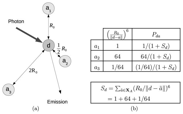
Figure 1 shows an example of the computation of P_da for a specific configuration of acceptors a around a donor d. The total probability that d de-excitates due to FRET is P_dA = Σ_a∈XA P_da. The probability that d de-excites by emission or by nonradiative decay is P_dD = 1 − P_dA.

Fig. 1.

(a) Donor fluorophore surrounded by three acceptors at distances R₀, $\frac{1}{2}{R}_0$ and 2R₀. (b) The table shows the de-excitation “path widths” (R₀/||d − a||)⁶ for energy transfer from the donor to each of the acceptors and the corresponding energy transfer probabilities P_da.

2.2. Model for intensities given protein configurations

Our model for the intensities given the configurations X_D and X_A is inspired by the model for simulation of FRET data in Corry, Jayatilaka and Rigby (2005). However, in contrast to Corry, Jayatilaka and Rigby (2005), we introduce the simplifying assumption that a donor or acceptor is always available for excitation [see also Wolber and Hudson (1979), Berney and Danuser (2003)]. This is a reasonable assumption if the intensity of the laser is moderate so that the inter arrival times of photons at a donor are large compared with the de-excitation times. We can then regard the times of excitations of donors and acceptors as Poisson processes and use standard results for Poisson processes to obtain closed-form distributional results for the $I_k^i$.

In the Appendix we show that $I_{DD}^i=G_D{N}_{DD}^i$ and $I_{DA}^i=G_A{N}_{DA}^i$, where $N_{DD}^i$ and $N_{DA}^i$ are the number of photons detected by the detector in, respectively, the DD-channel and the DA-channel, and $N_{DD}^i$ and $N_{DA}^i$ are both Poisson distributed. Further, G_D and G_A are unknown positive parameters related to the sensitivity of the detector in, respectively, the donor and acceptor emission spectrum. The means of $I_{DD}^i$ and $I_{DA}^i$ are

$${\mu }_{DD}^i=M_D\sum _{d\in {\mathbf{X}}_D\cap C_i}(1-P_{dA})$$

and

$${\mu }_{DA}^i=G{M}_D\sum _{a\in {\mathbf{X}}_A\cap C_i}\sum _{d\in {\mathbf{X}}_D}{P}_{da},$$

where M_D and G are unknown positive parameters. We assume that the means ${\mu }_{DD}^i/G_D$ and ${\mu }_{DA}^i/G_A$ of, respectively, $N_{DD}^i$ and $N_{DA}^i$ are sufficiently large so that the Poisson distributions of $N_{DD}^i$ and $N_{DA}^i$ can be well approximated by normal distributions. Then

$$I_{DD}^i~N({\mu }_{DD}^i,G_D{\mu }_{DD}^i)\text{and}{I}_{DA}^i~N({\mu }_{DA}^i,G_A{\mu }_{DA}^i).$$ (2.2)

By a similar line of arguments, we also obtain

$$I_{AA}^i~N({\mu }_{AA}^i,G_A{\mu }_{AA}^i),$$ (2.3)

where

$${\mu }_{AA}^i=(M_D/K)n({\mathbf{X}}_A\cap C_i),$$

K is an unknown positive parameter and n(X_A ∩ C_i) denotes the number of acceptors within pixel C_i. In cases of intensity data with a large proportion of zeros, we instead use truncated normal distributions with point masses at zero for $I_{DD}^i,I_{DA}^i$ and $I_{AA}^i$; see Section 2 of Supplement B [Hooghoudt and Waagepetersen (2017a)].

Equations (2.1), (2.2) and (2.3) specify the distribution of the FRET data conditional on the protein configurations X_D and X_A. The distribution is parameterized by ψ = (M_D, G, K, G_D, G_A, σ²). We refer to the components of ψ as microscope-related parameters. The parameters G and K are known as the so-called G- and K-factors [Zal, Zal and Gascoigne (2002), Chen, Puhl and Ikeda (2007)]. The parameter M_D can be interpreted as the mean donor emission detector read-out intensity due to one donor excitation.

3. Bayesian inference of spatial characteristics of protein configurations

We adopt a Bayesian approach to infer the microscope-related parameters ψ and spatial characteristics of the configurations X_D and X_A of proteins. A spatial point process prior (specified in Section 3.1) is used for X = (X_D, X_A), where this prior again depends on a parameter vector θ. We also assign a prior to θ, thus including also this parameter in the posterior inference. As detailed later in Sections 4.4 and 5, we recommend to infer the microscope-related parameters in an initial step using reference data without interactions between donors and acceptors. In a second step, investigating interactions in a dataset of biological scientific interest, ψ can then be fixed at estimates obtained from the first step. Letting y denote an observation of Y = (Y_DD, Y_DA, Y_AA) and (x_D, x_A) a realization of X, the joint posterior distribution is

$$p({\mathbf{x}}_D,{\mathbf{x}}_A,\theta \mid y,\psi )\propto p(y\mid {\mathbf{x}}_D,{\mathbf{x}}_A,\psi )p({\mathbf{x}}_D,{\mathbf{x}}_A\mid \theta )p(\theta ).$$ (3.1)

Here p(z) and p(z|u) are generic notation for a probability density of a random quantity Z and the conditional density of Z given another random quantity U = u.

3.1. Priors

We model a priori X_D and X_A as independent Poisson processes on W with intensities θ_D and θ_A; that is, the prior density of (X_A, X_D) with respect to independent unit rate Poisson processes is

$$p({\mathbf{x}}_D,{\mathbf{x}}_A\mid \theta )={\theta }_A^{n({\mathbf{x}}_A)}{\theta }_D^{n({\mathbf{x}}_D)}exp[-\mid W\mid ({\theta }_A+{\theta }_D-2)],$$ (3.2)

where |W| denotes the area of W and n(x) denotes the number of points in a point configuration x [see, for instance, equation (6.2) in Møller and Waagepetersen (2004)]. We further impose independent conjugate Gamma hyperpriors for θ_D and θ_A. The Poisson prior can be viewed as a null model for the case of no interaction between donors and acceptors or within donors, respectively, acceptors. Compared with other more complex point process models like Markov point processes (like the Strauss hard core model considered in Section 4), the Poisson prior is advantageous in having a known density function. A potential problem is that the Poisson prior is in some sense a strong prior which assigns little probability to point configurations with strong clustering or regularity. This can lead to biased results as demonstrated in Section 4. Densities for more flexible Markov point process prior models, on the other hand, contain intractable normalizing constants that depend on the unknown parameters in the point process model. This then precludes the use of standard Markov chain Monte Carlo algorithms (Section 3.2) for evaluation of the posterior distribution.

The Gamma distributions for θ_D and θ_A are defined through shape parameters α and rate parameters β. As the mean of the Gamma distribution is α/β and its variance α/β², the signal-to-noise ratio related to the distribution is defined by the square root of the shape parameter, that is,

$$\frac{S}{N}=\frac{\alpha /\beta }{\sqrt{\alpha /{\beta }^2}}=\sqrt{\alpha }.$$

In a typical FRET experiment there is quite some uncertainty concerning the true values of the numbers of proteins within the sample, and so we have defined not too confined priors for the intensities θ_D and θ_A. We have chosen to set the signal-to-noise ratio always equal to 2, resulting in the value of 4 for the shape parameter. In our applications we further specify the prior mean m of each of the parameters so that the rate parameter β follows from β = α/m = 4/m. We also use Gamma priors for the components of ψ; see the discussion of prior elicitation for ψ in Section 6.

3.2. Markov chain Monte Carlo

To evaluate the posterior distribution, we use a Markov chain Monte Carlo algorithm [Gamerman and Lopes (2006)] where the components (X_D, X_A), θ_D, θ_A and (if applicable) the components of ψ are updated in turn. Gibbs updates are used for the full conditional Gamma distributions of θ_D and θ_A, while random walk Metropolis updates on the log scale are used for the components of ψ. For the point configurations (X_A, X_D) we first randomly choose to either update X_A or X_D (with probability 1/2 for each choice). We then use birth-death updates as outlined in Sections 7.1.2–7.1.3 in Møller and Waagepetersen (2004). If, for example, X_A is chosen to be updated, then with probability 1/2 it is proposed to remove a point chosen from the uniform distribution on X_A. Otherwise it is proposed to insert a new acceptor point at a location chosen from the uniform distribution on W. In case it is proposed to remove a point u ∈ X_A, the Metropolis–Hastings ratio becomes

$$\frac{p({\mathbf{x}}_D,{\mathbf{x}}_A\backslash \{u\},\theta \mid y,\psi )n({\mathbf{x}}_A)}{p({\mathbf{x}}_D,{\mathbf{x}}_A,\theta \mid y,\psi )\mid W\mid }=\frac{p(y\mid {\mathbf{x}}_D,{\mathbf{x}}_A\backslash \{u\},\psi )n({\mathbf{x}}_A)}{p(y\mid {\mathbf{x}}_D,{\mathbf{x}}_A,\psi ){\theta }_A\mid W\mid }.$$

If it is proposed to insert a new acceptor point v ∈ W, then the Metropolis–Hastings ratio is

$$\frac{p(y\mid {\mathbf{x}}_D,{\mathbf{x}}_A\cup \{v\},\psi ){\theta }_A\mid W\mid }{p(y\mid {\mathbf{x}}_D,{\mathbf{x}}_A,\psi )(n({\mathbf{x}}_A)+1)}.$$

The expressions for updating X_D are similar. The described birth-death updates are repeated a large fixed number of times between the updates of the parameters θ_D, θ_A and ψ.

To keep the MCMC updates for donor and acceptor points numerically feasible, only those acceptors that reside within 4R₀ of a donor are taken into account as a possible path for energy transfer for the donor. This important simplification will not lead to any significant difference in posterior results, as the transfer probability P_da for a donor d and an acceptor a is very small when ||d − a|| > 4R₀, thereby adding or removing a point in pixel i can only affect the values of likelihood factors $p(y_{DD}^l,y_{DA}^l,y_{AA}^l\mid {\mathbf{x}}_D,{\mathbf{x}}_A,\psi )$ for pixels l in a neighborhood of i [note that the likelihood factors as ${\prod }_{i\in \mathcal{G}}p(y_{DD}^i,y_{DA}^i,y_{AA}^i\mid {\mathbf{x}}_D,{\mathbf{x}}_A,\psi )$]. Exploiting this simplification, we have implemented an ingenious algorithm that recomputes the transfer probabilities P_da only for donors and acceptors which are influenced by the adding/removing of a point. A detailed description of the MCMC sampler is provided in Supplement B [Hooghoudt and Waagepetersen (2017a)].

3.3. Inferring spatial characteristics

In statistics for spatial point processes, the K-function is a common tool for inferring interactions from a spatial point pattern. We adapt this approach and use the cross K-function [e.g., Møller and Waagepetersen (2004)] to measure interactions between donors and acceptors given point configurations x_A and x_D. In general, for point processes X₁ and X₂ of intensities ρ₁ and ρ₂, ρ₂K₁₂(t) is the expected number of X₂ points within distance t from a typical point of X₁. In case of no interaction between X₁ and X₂, K₁₂(t) = πt². Values of K₁₂(t) greater (smaller) than πt² signifies positive (negative) interaction between X₁ and X₂. It is common to consider the cross L-function $L_{12}(t)=\sqrt{K_{12}(t)/\pi }$ which is equal to t in the case of no cross interaction, while L₁₂(t) > t [L₁₂(t) < t] means positive (negative) cross interactions. We will refer to L₁₂(t) − t as the “centered” cross L-function. The centered cross L-function is equal to zero in the case of no cross interaction, while larger (smaller) than zero for positive (negative) cross interactions.

Given configurations x_D and x_A of donors and acceptors, we estimate the cross K-function by

$${\widehat{K}}_{\mathbf{x}}(t)=\sum _{u\in {\mathbf{x}}_A,v\in {\mathbf{x}}_D}\frac{1[\Vert u-v\Vert \le t]}{n({\mathbf{x}}_A)n({\mathbf{x}}_D)\mid W\cap W_{u-v}\mid {\mid W\mid }^{-2}},$$

where W_{u − v} is W translated by u − v [e.g., Section 4.4.3 in Møller and Waagepetersen (2004)]. The cross L-function is estimated by ${\widehat{L}}_{\mathbf{x}}(t)=\sqrt{{\widehat{K}}_{\mathbf{x}}(t)/\pi }$. To infer cross spatial interactions between donors and acceptors given FRET data, we consider the posterior distribution of ${\widehat{L}}_{\mathbf{X}}(t)=\sqrt{{\widehat{K}}_{\mathbf{X}}(t)/\pi }$ or its centered version. We also considered so-called cross G- and J -functions [e.g., Møller and Waagepetersen (2004)], but in our simulation studies the cross L-function gave a more clear impression of the nature of donor–acceptor interactions.

4. Simulation studies

Our primary target of inference is the cross L-function, L̂_X for the configuration X = (X_A, X_D) of donors and acceptors which is unknown in practice. However, we also need to infer the microscope-related parameters ψ. From a Bayesian perspective, if the right prior distribution is chosen, the posterior distribution by definition provides the correct inference given the data Y and prior information. However, in our case, the Poisson prior (3.2) is partly chosen for convenience in order to yield tractable MCMC computations, and is not necessarily the best possible representation of prior information. Thus, from a pragmatic point of view, it makes sense to assess possible bias of our Bayesian inference procedure.

In particular, we focus in Section 4.3.1 on the posterior mean L_|Y of L̂_X as a predictor of L̂_X. The posterior mean L_|Y is further an estimate of L^E = E[L̂_X], which is the expected value of L̂_X over replicated data X. Note in this connection that had we used the true distribution of X as the prior, then EL_|Y and L^E would be exactly equal—that is, L_|Y would be an unbiased predictor/estimate both of L̂_X and L^E. In Section 4.3.3 we assess the performance of the full posterior distribution of L̂_X given Y for inference regarding L̂_X. In Section 4.3 we consider ψ to be a fixed known parameter. Section 4.4 is concerned with inference regarding ψ.

4.1. Simulation of synthetic data

To generate synthetic data for the simulation study, the point configuration X = (X_A, X_D) is generated on a 1000 nm by 1000 nm square region as a realization of a bivariate Strauss hard core process. This point process has density (with respect to a bivariate process of independent unit rate Poisson processes) of the form

$$f({\mathbf{x}}_A,{\mathbf{x}}_D)\propto {\beta }_D^{n({\mathbf{x}}_D)}{\beta }_A^{n({\mathbf{x}}_A)}{\gamma }^{s_R({\mathbf{x}}_A,{\mathbf{x}}_D)}\text{HC}({\mathbf{x}}_A,{\mathbf{x}}_D,{\mathfrak{R}}_A,{\mathfrak{R}}_D,{\mathfrak{R}}_{DA}),$$ (4.1)

where s_R(x_A, x_D) is the number of unordered pairs of points {u, v} with u ∈ x_A, v ∈ x_D, and interpoint distance ||u − v|| less than R. Values of γ less than one lead to repulsion between donors and acceptors, while values of γ greater than one lead to attraction. The term HC(x_A, x_D, ℜ_A, ℜ_D, ℜ_DA) is one if the following hard core condition is satisfied: all donors have an interpoint distance greater than ℜ_D, all acceptors have an interpoint distance greater than ℜ_A, and all pairs of points where one is a donor and the other an acceptor have an interpoint distance greater than ℜ_DA. Otherwise the hard core term is zero, whereby it serves to model that donors and acceptors have a physical extent that prevents them from getting arbitrarily close to each other. Different settings of the Strauss hard core process parameters are used to create different point pattern types described in Section 4.2 below.

Next, conditional on the configuration X and the various microscope-related parameters ψ, the intensity data Y is generated from the model specified in Section 2. Regarding the observation model, we fix the measurement variance σ² at 25, let each of G, K, G_D, G_A equal to 1, and consider values 1, 5, 20 of M_D in order to generate data of varying signal to noise ratios defined by $\mathbf{E}[{\mu }_{DD}^i/{(G_D{\mu }_{DD}^i+{\sigma }^2)}^{1/2}]$ and $\mathbf{E}[{\mu }_k^i/{(G_A{\mu }_k^i+{\sigma }^2)}^{1/2}]$, k = DA, AA. For each point pattern type we generate 100 independent synthetic point patterns X^synth,i and associated synthetic image data Y^synth,i, i = 1, …, 100.

4.2. Point pattern types

The basic point pattern types considered are dimer, clustered, Poisson hard core and repulsive. For all types, ℜ_D, ℜ_A and ℜ_DA are at least 2 nm. The parameters β_D and β_A are further adjusted to have on average 1000 donors and 1000 acceptors.

In case of dimer, we specify large values of ℜ_D =ℜ_A, which essentially means that only proteins of different types can appear close to each other. Thus the only clusters possible are mini-clusters consisting of one donor and one acceptor, that is, dimer clusters. For the clustered case, ℜ_D = ℜ_A are reduced, which enables formation of a wider range of clusters containing several donors and acceptors. In case of dimer and clustered, values of γ_DA = 2, 8 correspond to respectively moderate and strong interactions. For Poisson hard core, γ_DA = 1, while all hard core distances are 2. In case of repulsive, varying values of ℜ_DA, r and γ_DA < 1 generate different strengths of repulsive interaction between donors and acceptors. Table 1 gives an overview of the different parameter settings considered.

Table 1.

Parameter settings used in the Strauss hard core model (4.1) to create the various point pattern types. The values for the homo (ℜ_DD, ℜ_AA) and hetero (ℜ_DA) hard core distances and the hetero interaction radius (R) presented in the table follow from the considerations stated in the text and by the choice of the Förster distance R₀ = 6

Type number	ℜDD =ℜAA	ℜDA	R	γDA	Short name
1	18	2	6	2	Dim.12
2	18	2	6	8	Dim.18
3	12	2	6	2	Dim.22
4	12	2	6	8	Dim.28
5	6	2	6	2	Clu.12
6	6	2	6	8	Clu.18
7	2	2	6	2	Clu.22
8	2	2	6	8	Clu.28
9	2	2	0	1.0	Poi.HC
10	2	6	0	1.0	Rep.h1
11	2	12	0	1.0	Rep.h2
12	2	2	10	0.5	Rep.s1
13	2	2	10	0.1	Rep.s2

4.3. Inference regarding spatial characteristics

We estimate L^E by the empirical average of L-functions L̂_X^synth,i obtained from the X^synth,i. From each synthetic dataset Y^synth,i we further obtain an MCMC estimate L̄_|Y^synth,i of the posterior mean L_|Y^synth,i of L̂_X given Y^synth,i. The mean posterior L-function EL_|Y is estimated by the mean of the L̄_|Y^synth,i. The sampling variability of L_|Y is further represented by the variation of the L̄_|Y^synth,i. When considering inference for the cross L-function in the following Sections 4.3.1–4.3.3, ψ is fixed at the value used for generating the synthetic datasets.

4.3.1. Bias of posterior mean

We assess the bias of L_|Y by considering the mean (over replicated data X,Y) of L̂_X and its prediction L_|Y, thereby we also assess how L_|Y performs as an estimate of L^E (the expected cross L-function for X).

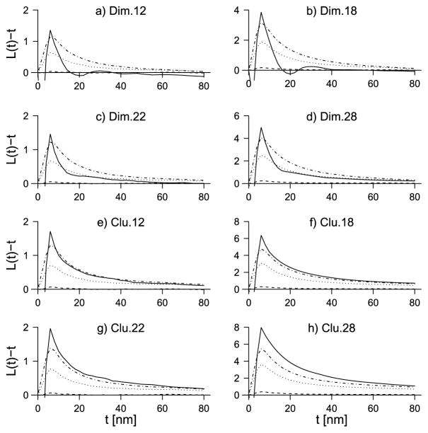
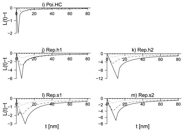
In Figures 2 and 3 the estimates of L^E(t) − t and EL_|Y (t) − t are shown for each of the point pattern types in Table 1 for the three values of M_D (1, 5, 20). In Figure 2(a), for example, L^E for dimer-type 1.2 shows that the underlying point patterns are clustered for distances r < 16 (as L^E > 0) and are slightly repulsive for distances 16 < r < 24. Further, for distances 24 < r < 40, there seems to be some slight clustering again, while, for r > 40, the pattern displays complete spatial randomness. The negative values that occur for r < 5 are due to the minimum imposed hardcore distance of 2. The negative part for small r is also visible in the plots (b)–(h), where L^E otherwise indicates clustering among donors and acceptors and in plot (i), where L^E(t) − t is close to zero otherwise.

Fig. 2.

In each plot the solid line is the centered L^E-function. The other lines show the centered EL_|Y for varying M_D: dashed line: M_D = 1, dotted line: M_D = 5, dashed-dotted line: M_D = 20. The plots are for the dimer and clustered point pattern types.

Fig. 3.

Continuation of Figure 2. Plots are for the Poisson hard core and repulsive types.

The general impression from the plots is that L_|Y is biased downward when the true point patterns are of dimer or clustered types (a)–(h) and biased upward in the cases of the repulsive types (i)–(m) (including the Poisson hard core case). For M_D = 1, where the signal-to-noise ratio is very low, the mean of L_|Y is very close to zero, and it does not seem possible to infer in this case cross interactions between donors and acceptors. However, for M_D = 5, 20, there is always a pronounced peak (positive or negative) of the mean L_|Y-function where the peak is of the right sign and located in the right place of the peak of the L^E-function. Moreover, the bias consistently decreases when M_D and hence the signal-to-noise ratio increases. Despite the bias, the results suggest that qualitatively correct statements can be made regarding independence, clustering or repulsion between donors and acceptors.

4.3.2. Variability of posterior mean L-function

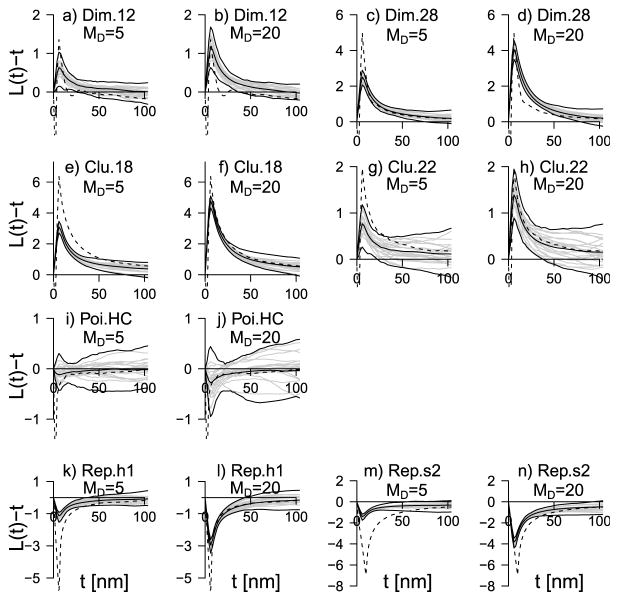
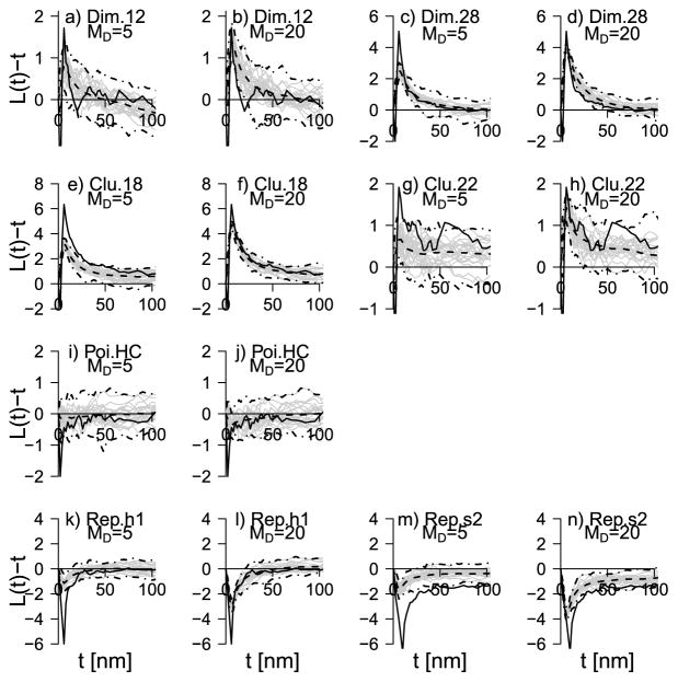
In addition to bias, the extent to which valid qualitative conclusions can be made from the posterior L_|Y-function of course also depend on its variability. Figure 4 shows for each basic point pattern type and M_D either 5 or 20, 98% envelopes for L_|Y (t) based for each t on the minimal and maximal values of L_|Y (t) over the 100 replications. These envelopes are fairly narrow for distances up to 100 and show that, in the setting of the simulation study, qualitative conclusions regarding the nature of interaction between donors and acceptors will be consistently correct over replicates.

Fig. 4.

Distribution of the centered L̄_|Y-function for the various point pattern types, summarized by 98% envelopes based on L̄_|Y^synth,i, i = 1, …, 100, together with the mean value ÊL_|Y (middle solid line). The value of M_D is 5 or 20. In each plot twenty of the L̄_|Y^synth,i’s are shown with solid gray curves, the dashed line is the centered L̂^E-function.

4.3.3. Inference based on full posterior distribution

The results in Section 4.3.1 showed that the posterior mean L-function L_|Y can exhibit substantial bias as an estimate of L^E and hence also as a predictor of L̂_X. This can invalidate the use of the full posterior distribution for inferring the uncertainty regarding the estimation of L^E or the prediction of L̂_X. As an example Figure 5 shows L_|Y^synth,1(t) − t and the 98% central posterior interval for L̂_X(t) − t given Y = Y_synth,1 for the same point pattern types as in Figure 4 and M_D = 5, 20. Also, the true L̂_X^synth,1(t) − t are shown in each plot.

Fig. 5.

Posterior distribution of L̂_X given the first synthetic dataset Y^synth,1 for each point pattern type. Dashed: posterior mean L_|Y^synth,1, dashed-dotted: 98% envelopes and solid gray: twenty posterior realizations of L̂_X. Solid black shows the true L̂_X^synth,1.

For the lower signal-to-noise ratio with M_D = 5, L̂_X^synth,1(t) falls outside the 98% posterior interval for several point pattern types. Thus the posterior intervals do not always give a useful quantification of the uncertainty regarding the knowledge of L_X. However, for the higher signal-to-noise ratio with M_D = 20, the envelopes do include or almost include the L̂_X^synth,1 function.

4.4. Simulation studies for microscope parameters

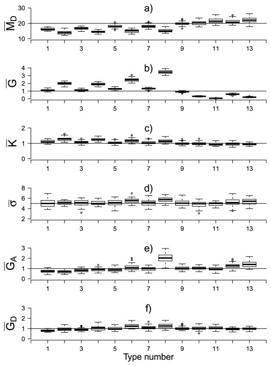
So far the vector ψ of microscope-related parameters has been assumed to be known, which is rarely the case. We have investigated Bayesian inference for ψ in a simulation study for which the full details are given in Supplement C [Hooghoudt and Waagepetersen (2017b)]. We here just comment on results obtained for simulations with G_D = G_A = K = G = 1, M_D = 20 and σ² = 25. Figure 6 shows boxplots of the posterior mean of each microscope parameter over 40 replicated datasets for each point pattern type. The main features are as follows:

Fig. 6.

Boxplots of the posterior mean of all the six microscope parameters for the forty replicated runs for each of the point pattern types (referred to by their type number, see Table 1) for $M_D^s=20$. The horizontal lines are drawn at the corresponding synthetic values.

1. for the Poisson hard core patterns the posterior means of all the parameters coincide with or are very close to their respective synthetic values [see plots (a)–(f) for type number 9].

2. for all the clustered patterns (type number 1–8) inference for M_D,G and K is biased. The posterior means M̄_D are significantly below their synthetic value, while Ḡ and K̄ are above their target values. Further, the bias increases for the patterns generated with γ_DA = 8 (type number 2, 4, 6, 8) compared to the corresponding patterns generated with γ_DA = 2 (type number 1, 3, 5, 7).

3. for repulsive patterns (type number 11–13) M̄_D and K̄ are on or close to target, while Ḡ is negatively biased.

4. the posterior means of σ, G_A and G_D are on target for almost all point pattern types [plots (d)–(f)].

As explained in detail in Supplement C, the biased results are due to the mismatch between the Poisson point process prior and the actual point processes used for the simulations. The microscope-related parameters thus a posteriori take on values to “soothe” this mismatch, resulting in biased results. Further, in this setting with joint inference of ψ and spatial characteristics, the posterior mean L-functions are strongly biased as well, being close to zero for all distances for all point pattern types (not shown).

5. Two-step approach to likelihood-based inference

In the previous Section 4.4 we observed that applying the Bayesian inference methodology using the Poisson process prior on Poisson hard core patterns gave reliable estimates for all microscope parameters. This suggests an approach where microscope-related parameters are inferred from reference datasets constructed with absence of donor–acceptor interactions. Therefore, we propose a two-step approach where the microscope-related parameters are inferred in a first step using reference data. In the second step the values of the microscope parameters are fixed at the posterior estimates from the first step in order to make inference on the spatial configuration of donors and acceptors of a three-cube FRET sample of biological scientific interest. To illustrate the approach, we have carried out the first step on empirical reference three-cube FRET data, as discussed in the following section.

6. Data example

In this section we apply our Bayesian methodology to empirical in vitro three-cube FRET data obtained from donor or acceptor fluorophore labeled transferrin proteins [Welch (1992)] attached to polylysine slides [Shima and Sakai (1977)]. Transferrin bound to polylysine is known to be approximately randomly (i.e., Poisson hardcore) distributed [Wallrabe et al. (2007)]. The objective is to infer the microscope parameters related to the experimental setup.

We initially conducted an exploratory analysis [described in Supplement A, Hooghoudt, Barroso and Waagepetersen (2017)] where we quantified the amount of photobleaching and compared empirical mean–variance relationships of the image data with the ones implied by our model. From these mean–variance relationships, as well as other non-Bayesian methods discussed in Supplement A, we obtained rough estimates for the microscope parameters that were used to set the prior means in the Bayesian analysis. We thus use a pragmatic Bayesian approach where the rough non-Bayesian estimates entering in the priors are refined by introducing information obtained through the likelihood derived from our observation model.

Due to certain computational issues discussed in Section 6.2 and Section 6.3.1, we are at this stage only able to use a small subset of the full data in the Bayesian inference. Improving the computational methodology is an important topic of further research.

6.1. The image dataset

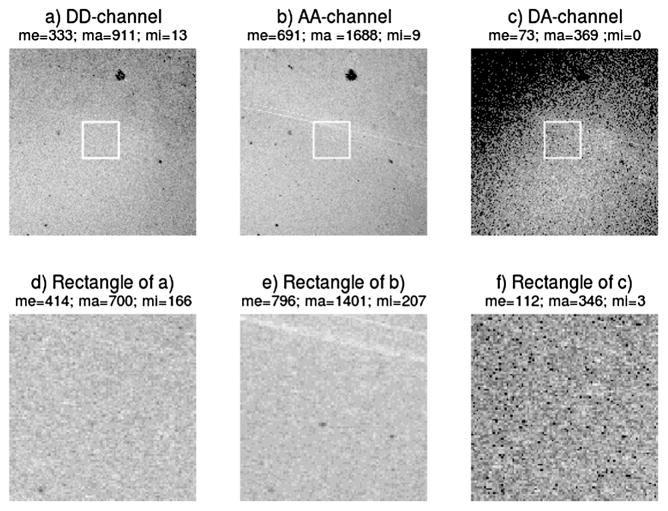
Three cube FRET measurements have been carried out on three samples, to which we refer as samples 1, 2 and 3. Sample 1 is prepared to consist of twice as many donors (D) as acceptors (A), that is, $\mathrm{D}:\mathrm{A}\approx 1:\frac{1}{2}$, while samples 2 and 3 are prepared such that, respectively, D : A ≈ 1 : 1 and $\mathrm{D}:\mathrm{A}\approx \frac{1}{2}:1$. Three-cube FRET data is obtained on each sample on a square grid containing 512 × 512 square pixels. The pixel side length is 0.279 μm and the focal volume depth is approximately 5 pixels (1.4 μm) [Wallrabe et al. (2007)]. The image data are shown in Figure 7.

Fig. 7.

Channel intensity images of the aggregated channel dataset of sample 2. (a) DD-channel, (b) AA-channel, (c) DA-channel. Plots (a)–(c) consist each of 512 × 512 pixels. Plots (d)–(f) show enlargements of the square subregions of the plots (a)–(c), each consisting of 100×100 pixels. Above each plot is stated the mean (me), maximum (ma) and minimum (mi) pixel intensity value in the image. In each image the gray levels are constructed by using ten equally spaced intervals between zero and the maximum value of the image. Black/white refers to the lowest/highest intensity interval.

The emission in the DD-channel (Y_DD) and AA-channel (Y_AA) are corrected for background emission, while the DA-channel data (Y_DA) is also corrected for spectral bleedthrough by the methods described in Elangovan et al. (2003).

We noticed that around the edges of the 512 × 512 images, often very low or zero intensity regions occurred due to improper sample preparation. Therefore, the exploratory statistical analysis has been based solely on the central rectangular section of the images consisting of 100 × 100 pixels (see also Supplement A, Section 1).

In order to obtain sufficient photon count statistics—that is, sufficiently high signal-to-noise ratio for each pixel—each sample has been remeasured ten times. We then create an aggregated dataset by summing pixelwise over the ten measured intensities for each channel. We note that by remeasuring the sample instead of increasing the measurement time, we obtain information concerning the amount of photobleaching occurring for remeasurements (Supplement A, Section 3) and the pixel intensity variance in the three channels. The latter information gives the possibility to deduce the empirical mean–variance relationship of the image data and to obtain estimates for G_D and G_A (Supplement A, Section 6).

6.2. Inference procedure setup

The prior distributions for the microscope and Poisson point process parameters were specified as Gamma distributions. For each parameter the shape parameter is set to 4 based on the reasoning in Section 3.1, and we use a pragmatic Bayesian approach where the prior means of five of the microscope parameters are set by aid of the rough estimates M_D ≈ 2.6, G ≈ 0.7, K ≈ 0.7, G_D ≈ 7.4 and G_A ≈ 5.5 obtained from the preliminary statistical analysis in Supplement A, Sections 3–6 and 8. The prior mean of the measurement noise σ² we have set, rather ad hoc, to 50.

By the statistical analysis in Section 8 of Supplement A, it was further found that the point process intensities θ_A and θ_D of the samples can be roughly related to the donor and acceptor solution concentrations applied for the sample preparation, thereby we found that, for sample 1, θ_D ≈ 2e3 μm⁻² and θ_A ≈ 1e3 μm⁻²; while, for sample 2, θ_D ≈ 2e3 μm⁻² and θ_A ≈ 2e3 μm⁻²; and, for sample 3, θ_D ≈ 1e3 μm⁻² and θ_A ≈ 2e3 μm⁻².We use these values as prior means for θ_A and θ_D for each of the samples. The applied prior means as used in the Bayesian analyses are summarized in Table 2.

Table 2.

Prior means for the microscope parameters and the Poisson point process intensities, as well as the values of the tuning parameter τ applied to generate proposals for the microscope parameters

	Samples 1, 2 and 3						Sample 1		Sample 2		Sample 3
	MD	G	K	GD	GA	σ2	θD	θA	θD	θA	θD	θA
Prior mean	2.5	1.0	1.0	5.0	5.0	50.0	2e3	1e3	2e3	2e3	1e3	2e3
τ	0.05	0.1	0.1	0.5	0.5	1.0	–	–	–	–	–	–

In the MCMC computations we used random walk Metropolis–Hastings updates for the log microscope-related parameters. The values of the random walk update standard deviations τ are also shown in Table 2. We tuned the τ values to get an approximately 30% proposal acceptance rate for each of the microscope parameters. The total number of MCMC updates is 5e9 for each run. Metropolis– Hastings updates for the microscope parameters and Gibbs updates for the point process parameters are made after every 1e4 birth/death updates of donor or acceptor points.

The MCMC chains converge slowly due to bad mixing as discussed in Section 6.3. This means that we need many rounds of birth-death updates for the donor/acceptor points followed by updates of microscope and point process parameters. In each round we need to update a large fraction of the donors and acceptors. Thus, for a fixed fraction, each round takes more computing time the higher posterior expected number of donors and acceptors. The a posteriori expected number of donors and acceptors in each pixel is fairly high (of the order 300). To keep the computation time at an acceptable level, we therefore perform the inference on a small 10×10 subset of pixels which contain a posteriori of the order of 3e4 donors and acceptors.

6.3. Results of the inference

6.3.1. Assessment of MCMC samples

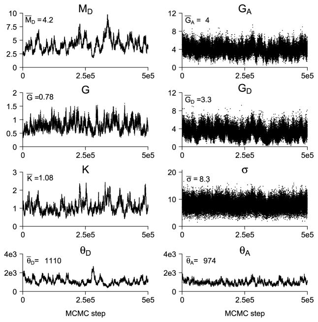
In Figure 8 the traceplots of the microscope parameters and the Poisson point process intensities for sample 1 are shown. Posterior mean values are displayed in the upper left corner of each of the plots. The traceplots indicate poor mixing of the MCMC samples except for G_A, G_D and σ.

Fig. 8.

Traceplots of the microscope and the Poisson point process parameters for sample 1. Posterior mean values are displayed in the upper left corner of each of the plots. For plotting a subsampling of 10 has been applied.

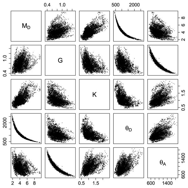
The poor mixing is due to high posterior correlation between certain parameters as visualized by the scatterplots in Figure 9 in which the posterior realizations of M_D, G, K, θ_D, θ_A are plotted against each other. Especially M_D and θ_D and G and θ_A are highly correlated, but fairly strong correlations are also evident between M_D and K and between K and θ_D. Similar scatterplots of G_D, G_A and σ² versus each of the other parameters (not shown) do not show any clear correlation with any of the parameters.

Fig. 9.

Scatterplots of the posterior realizations of M_D,G,K, θ_D, θ_A versus each other for sample 1. For plotting a subsampling of 100 has been applied.

6.3.2. Posterior results

InTable3 the 95% posterior intervals and posterior means for each of the microscope parameters and Poisson intensities are stated for each of the three samples. The microscope parameters M_D, G, G_A, G_D and σ should be equal for all samples, and this may seem contradicted by their posterior means that vary across samples. There is, on the other hand, considerable overlap between almost all 95% posterior intervals so that the Bayesian inference does not contradict that the microscope parameters are equal across samples.

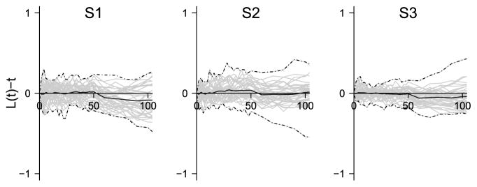
Figure 10 shows the posterior distributions of the centered L-function for the three samples. As expected, there is no indication of clustering nor repulsion since the centered posterior L-functions are close to zero and the posterior means are approximately zero.

Fig. 10.

Posterior distribution of the L-function for samples 1–3. For each sample the posterior distribution is summarized by the posterior mean (solid line) of the L-function and 95% envelopes based on minimal (lower dashed-dotted line) and maximal (upper dashed-dotted line) values of 39 posterior realizations of the L-function.

7. Discussion

This paper presents a first attempt to implement likelihood-based inference for FRET data. We thus, based on physical considerations, developed a realistic observational model for FRET data given the underlying configurations of donors and acceptors. Based on this model, we proposed to implement Bayesian inference using MCMC.

We quantify spatial dependence by considering the posterior mean of the cross L-function for the donors and acceptors. Our simulation results show that the posterior mean of the L-function can be used to distinguish between clustering, absence of interaction and repulsion between donors and acceptors. Due to bias, one needs to be careful when making quantitative statements regarding strength of interaction based on the posterior means of the L-functions. However, we believe that it is meaningful to make relative comparisons of strength of interactions between samples observed under the same experimental conditions and thus with the same signal-to-noise ratios.

Partly due to poor mixing of the proposed MCMC procedure, we were forced to consider only a small subset of the full data. A key objective for further research is therefore to obtain a more efficient MCMC scheme so that efficient use of the full data becomes feasible. Haario, Saksman and Tamminen (2001) suggest to use joint updates, but they consider posterior distributions of fixed dimensional random vectors. However, preliminary experiments with this approach indicate that we need joint updates involving both the microscope parameters and the donor-acceptor point patterns. It is not clear how to do this. Our data example illustrated the use of reference data with no donor–acceptor interactions to infer the microscope-related parameters. In future work it would interesting to apply an improved MCMC algorithm to conduct Bayesian inference for an experimental sample with possible interactions.

The Poisson point process prior for protein configurations was chosen partly for computational reasons. To implement Bayesian inference with more flexible Markov point process priors allowing for both repulsive and attractive interactions requires more advanced Markov chain Monte Carlo methods developed in Møller et al. (2006) and Murray, Ghahramani and MacKay (2006). However, these methods are highly computationally demanding since they involve so-called perfect simulation from the point process prior, which can lead to unacceptable computing times in the case of protein configurations of high cardinality which are frequently encountered for FRET data.

Supplementary Material

SuppC

Supplement C: Inference of the microscope parameters (DOI: 10.1214/17- AOAS1054SUPPC; .pdf). The supplementary material contains a detailed description of the inference of the microscope parameters.

SupplA

Supplement A: Preliminary statistical analysis of the in vitro three-cube FRET dataset (DOI: 10.1214/17-AOAS1054SUPPA; .pdf). The supplementary material contains a preliminary statistical analysis of the in vitro three cube FRET dataset. Sample preparation and experimental setup are discussed as well the channel dataset extracted from the samples. The amount of photobleaching for the remeasurements in the three channels is studied and the mean–variance relations of the dataset are compared with the ones given by our statistical model. Further, estimates for the microscope parameters are obtained through various non-Bayesian methods.

SupplB

Supplement B: The MCMC sampler (DOI: 10.1214/17-AOAS1054SUPPB; .pdf). The supplementary material contains a detailed description of the steps performed in the MCMC sampler.

Table 3.

Posterior results for each of the three samples: 95% posterior intervals and posterior means (in brackets) for each of the parameters. Prior means of the parameters are given in Table 2

	Sample
	1	2	3
MD	2.3–7.0 (4.2)	3.1–8.6 (5.5)	2.8–6.8 (4.7)
G	0.46–1.21 (0.78)	0.50–1.36 (0.89)	0.19–0.52 (0.32)
K	0.61–1.93 (1.08)	0.31–0.98 (0.60)	0.51–1.49 (0.92)
GA	1.9–6.2 (4.0)	5.3–12.7 (8.9)	8.0–13.4 (10.6)
GD	1.2–5.7 (3.3)	3.0–10.0 (6.3)	1.7–6.5 (3.9)
σ	4.4–12.0 (8.3)	3.8–10.7 (7.2)	4.2–11.6 (7.9)
θD	6.1e2–19.3e2 (11.1e2)	7.8e2–2282 (13.4e2)	9.0e2–23.5e2 (14.7e2)
θA	6.1e2–15.0e2 (9.7e2)	8.3e2–20.4e2 (12.8e2)	15.0e2–34.1e2 (23.5e2)

APPENDIX: DERIVATION OF OBSERVATION MODEL

In this section we refer to notation introduced in Section 2. Let L_d denote the set of times in the observation time span [0, T] where a donor d in X_D is excited by a photon from the laser. We assume that L_d is a homogeneous Poisson process on [0, T] with intensity λ_D > 0. The process L_d can be decomposed as

$$L_d=L_{dE}\cup L_{dN}\underset{a\in {\mathbf{X}}_A}{\cup }{L}_{da},$$

where L_dE denotes the times of excitations of d which resulted in emission in the D channel, L_dN is the times of excitations resulting in nonradiative de-excitation and L_da denotes the times of excitations that resulted in FRET to acceptor a and subsequent emission in the A channel. The so-called quantum yield 0 < q_D < 1 is the probability of emission for donors conditional on that de-excitation is by emission or nonradiatively, that is, q_D = k_DE/k_D. Similarly, q_A denotes the quantum yield for acceptors. Invoking the random labeling theorem for Poisson processes [e.g., Proposition 3.7 in Møller and Waagepetersen (2004)], L_dE, L_da and L_dN are independent Poisson processes with intensities λ_Dq_DP_dD, λ_Dq_AP_da and λ_D[(1 − q_D)P_dD +Σ_a∈XA(1− q_A)P_da].

For each i ∈ 𝒢 we let

$$L_{DD}^i=\underset{d\in {\mathbf{X}}_D\cap C_i}{\cup }{L}_{dE}$$

and

$$L_{DA}^i=\underset{d\in {\mathbf{X}}_D,a\in {\mathbf{X}}_A\cap C_i}{\cup }{L}_{da}$$

be the Poisson processes of donor excitation times which result in photon emissions for respectively donors and acceptors in the pixel C_i.

The emitted photons fall on the detector independently of each other with a probability 0 < h < 1 of detection. In the point process literature the detected photons are called an independent thinning with retention probability h. Further, of the detected photons only independent thinnings with retention probabilities 0 < Q_D < 1 (0 < Q_A < 1) are registrated in the donor (acceptor) channel of the detector. The probabilities Q_D and Q_A are respectively the detector quantum yields in the donor and acceptor channel [Pawley (2006)]. The detected photon counts $N_{DD}^i$ and $N_{DA}^i$ of emissions in the pixel C_i are thus Poisson distributed with means Q_Dhq_Dλ_DT Σ_d∈XD∩Ci P_dD and Q_Dhq_Aλ_DT Σ_{d∈XD,a∈XA∩Ci} P_da. Finally, $I_{DD}^i=G_D{N}_{DD}^i$ and $I_{DA}^i=G_A{N}_{DA}^i$, where G_D and G_A are amplification factors depending on the detector and channel. Defining M_D = G_DQ_Dhq_Dλ_DT and G = (G_AQ_Aq_A)/(G_DQ_Dq_D), we arrive at the specified means of $I_{DD}^i$ and $I_{DA}^i$.

The mean of $I_{AA}^i$ is found in a similar fashion. In the AA-channel acceptors are directly excited by the laser which is now broadcasting in the acceptor excitation spectrum with an intensity λ_A > 0. An excited acceptor can only de-excite due to emission or nonradiatively, and the detected photon counts $N_{AA}^i$ of emissions in the pixel C_i are Poisson distributed with means Q_Ahq_Aλ_AT Σ_a∈XA∩Ci 1 and $I_{AA}^i=G_A{N}_{AA}^i$. Defining M_A = G_AQ_Ahq_Aλ_AT and K = M_D/M_A, we arrive at the specified mean of $I_{AA}^i$.

References

- Alber F, Dokudovskaya S, Veenhoff LM, Zhang W, Kipper J, Devos D, Suprapto A, Karni-Schmidt O, Williams R, Chait BT, Rout MP, Sali A. Determining the architectures of macromolecular assemblies. Nature. 2017;450:683–694. doi: 10.1038/nature06404. [DOI] [PubMed] [Google Scholar]
- Berney C, Danuser G. FRET or no FRET: A quantitative comparison. Biophys J. 2003;84:3992–4010. doi: 10.1016/S0006-3495(03)75126-1. [DOI] [PMC free article] [PubMed] [Google Scholar]
- Bonomi M, Pellarin R, Kim SJ, Russel D, Sundin BA, Riffle M, Jaschob D, Ramsden R, Davis TN, Muller EGD, Sali A. Determining protein complex structures based on a Bayesian model of in vivo Förster resonance energy transfer data. Mol Cell Proteomics. 2014;13:2812–2823. doi: 10.1074/mcp.M114.040824. [DOI] [PMC free article] [PubMed] [Google Scholar]
- Bunt G, Wouters FS. Visualization of molecular activities inside living cells with fluorescent labels. Int Rev Cytol. 2004;237:205–277. doi: 10.1016/S0074-7696(04)37005-1. [DOI] [PubMed] [Google Scholar]
- Chen H, Puhl HL, III, Ikeda SR. Estimating protein–protein interaction affinity in living cells using quantitative Förster resonance energy transfer measurements. J Biomed Opt. 2007;12 doi: 10.1117/1.2799171. Art. ID 054011. [DOI] [PubMed] [Google Scholar]
- Chen LC, Lloyd WR, III, Chang CW, Sud D, Mycek MA. Fluorescence lifetime imaging microscopy for quantitative biological imaging. Digital Microscopy. In: Sluder G, Wolf DE, editors. Methods in Cell Biology. Vol. 114. Academic Press; San Diego, CA: 2013. pp. 457–488. [DOI] [PubMed] [Google Scholar]
- Clegg RM. Fluorescence resonance energy transfer. Curr Opin Biotechnol. 1995;6:103–110. doi: 10.1016/0958-1669(95)80016-6. [DOI] [PubMed] [Google Scholar]
- Clegg RM. The history of FRET. In: Geddes CD, Lakowicz JR, editors. Reviews in Fluorescence. Springer; New York: 2006. pp. 1–45. [Google Scholar]
- Corry B, Jayatilaka D, Rigby P. A flexible approach to the calculation of resonance energy transfer efficiency between multiple donors and acceptors in complex geometries. Biophys J. 2005;89:3822–3836. doi: 10.1529/biophysj.105.069351. [DOI] [PMC free article] [PubMed] [Google Scholar]
- Elangovan M, Wallrabe H, Chen Y, Day RN, Barroso M, Periasamy A. Characterization of one- and two-photon excitation fluorescence resonance energy transfer microscopy. Methods. 2003;29:58–73. doi: 10.1016/s1046-2023(02)00283-9. [DOI] [PubMed] [Google Scholar]
- Erickson HP. Size and shape of protein molecules at the nanometer level determined by sedimentation, gel filtration, and electron microscopy. Biol Proced Online. 2009;11:32–51. doi: 10.1007/s12575-009-9008-x. [DOI] [PMC free article] [PubMed] [Google Scholar]
- Förster Th. Zwischenmolekulare Energiewanderung und Fluoreszenz. Ann Phys. 1948;437:55–75. doi: 10.1002/andp.19484370105. [DOI] [Google Scholar]
- Frederix PL, de Beer EL, Hamelink W, Gerritsen HC. Dynamic Monte Carlo simulations to model FRET and photobleaching in systems with multiple donor–acceptor interactions. J Phys Chem B. 2002;106:6793–6801. [Google Scholar]
- Gamerman D, Lopes HF. Markov Chain Monte Carlo: Stochastic Simulation for Bayesian Inference. 2. Chapman & Hall/CRC; Boca Raton, FL: 2006. MR2260716. [Google Scholar]
- Gilks WR, Richardson S, Spiegelhalter DJ, editors. Markov Chain Monte Carlo in Practice. Chapman & Hall; London: 1996. MR1397966. [Google Scholar]
- Goswami D, Gowrishankar K, Bilgrami S, Ghosh S, Raghupathy R, Chadda R, Vishwakarma R, Rao M, Mayor S. Nanoclusters of GPIanchored proteins are formed by cortical Actin-driven activity. Cell. 2008;135:1085–1097. doi: 10.1016/j.cell.2008.11.032. [DOI] [PMC free article] [PubMed] [Google Scholar]
- Gryczynski Z, Gryczynski I, Lakowicz JR. Molecular Imaging: FRET Microscopy and Spectroscopy. Elsevier; Amsterdam: 2005. Basics of fluorescence and FRET; pp. 21–56. [Google Scholar]
- Haario H, Saksman E, Tamminen J. An adaptive Metropolis algorithm. Bernoulli. 2001;7:223–242. MR1828504. [Google Scholar]
- Heitler W. The Quantum Theory of Radiation. Dover; New York: 1954. [Google Scholar]
- Hooghoudt J-O, Barroso M, Waagepetersen R. Supplement A: Preliminary statistical analysis of the three-cube FRET dataset. 2017 doi: 10.1214/17-AOAS1054SUPPA. [DOI] [Google Scholar]
- Hooghoudt J-O, Waagepetersen R. Supplement B: The MCMC sampler. 2017a doi: 10.1214/17-AOAS1054SUPPB. [DOI] [Google Scholar]
- Hooghoudt J-O, Waagepetersen R. Supplement C: Inference of the microscope parameters. 2017b doi: 10.1214/17-AOAS1054SUPPC. [DOI] [Google Scholar]
- Kenworthy AK. Imaging protein–protein interactions using fluorescence resonance energy transfer microscopy. Methods. 2001;24:289–296. doi: 10.1006/meth.2001.1189. [DOI] [PubMed] [Google Scholar]
- Kenworthy AK, Edidin M. Distribution of a Glycosylphosphatidylinositol-anchored protein at the apical surface of MDCK cells examined at a resolution of <100 Å using imaging fluorescence resonance energy transfer. J Cell Biol. 1998;142:69–84. doi: 10.1083/jcb.142.1.69. [DOI] [PMC free article] [PubMed] [Google Scholar]
- Krissinel E, Henrick K. Inference of macromolecular assemblies from crystalline state. J Mol Biol. 2007;372:774–797. doi: 10.1016/j.jmb.2007.05.022. [DOI] [PubMed] [Google Scholar]
- Lakowicz JR. Principles of Fluorescence Spectroscopy. Springer; New York: 2009. [Google Scholar]
- Loura LMS, Fernandes F, Prieto M. Membrane microheterogeneity: Förster resonance energy transfer characterization of lateral membrane domains. Eur Biophys J. 2010;39:589–607. doi: 10.1007/s00249-009-0547-5. [DOI] [PubMed] [Google Scholar]
- Loura LMS, Prieto M. FRET in membrane biophysics: An overview. Front Physiol. 2011;2 doi: 10.3389/fphys.2011.00082. Art. ID 82. [DOI] [PMC free article] [PubMed] [Google Scholar]
- Miyawaki A, Sawano A, Kogure T. Lighting up cells: Labelling proteins with fluorophores. Nat Cell Biol. 2003;5:S1–S7. [PubMed] [Google Scholar]
- Møller J, Waagepetersen RP. Monographs on Statistics and Applied Probability. Chapman & Hall/CRC; Boca Raton, FL: 2004. Statistical Inference and Simulation for Spatial Point Processes; p. 100. MR2004226. [Google Scholar]
- Møller J, Pettitt AN, Reeves R, Berthelsen KK. An efficient Markov chain Monte Carlo method for distributions with intractable normalising constants. Biometrika. 2006;93:451–458. MR2278096. [Google Scholar]
- Murray I, Ghahramani Z, MacKay DJC. MCMC for doubly-intractable distributions. Proceedings of the 22nd Annual Conference on Uncertainty in Artificial Intelligence (UAI-06); Arlington, VA: AUAI Press; 2006. pp. 359–366. [Google Scholar]
- Pawley J. Handbook of Biological Confocal Microscopy. Springer; New York: 2006. [Google Scholar]
- Periasamy A, Day R, editors. Molecular Imaging: FRET Microscopy and Spectroscopy. Elsevier; Amsterdam: 2011. [Google Scholar]
- Periasamy A, Wallrabe H, Chen Y, Barroso M. Quantitation of protein– protein interactions: Confocal FRET microscopy. Biophysical Tools for Biologists, Volume Two: In Vivo Techniques. In: Correia JJ, Detrich HWI, editors. Methods in Cell Biology. Vol. 89. Academic Press; San Diego, CA: 2008. pp. 569–598. [DOI] [PubMed] [Google Scholar]
- Polo SE, Jackson SP. Dynamics of DNA damage response proteins at DNA breaks: A focus on protein modifications. Genes Dev. 2011;25:409–433. doi: 10.1101/gad.2021311. [DOI] [PMC free article] [PubMed] [Google Scholar]
- Puglisi JD. NATO Science Series, I: Life and Behavioural Sciences. IOS Press; Amsterdam: 2005. Structure, Dynamics and Function of Biological Macromolecules and Assemblies; p. 364. [Google Scholar]
- Raicu V, Stoneman MR, Fung R, Melnichuk M, Jansma DB, Pisterzi LF, Rath S, Fox M, Wells JW, Saldin DK. Determination of supramolecular structure and spatial distribution of protein complexes in living cells. Nat Photonics. 2009;3:107–113. [Google Scholar]
- Rohatgi-Mukherjee KK. Fundamentals of Photochemistry. Wiley; New Delhi: 1978. [Google Scholar]
- Shima S, Sakai H. Polylysine produced by Streptomyces. Agric Biol Chem. 1977;41:1807–1809. [Google Scholar]
- Sun Y, Wallrabe H, Seo SA, Periasamy A. FRET microscopy in 2010: The legacy of Theodor Förster on the 100th anniversary of his birth. Chemphyschem. 2011;12:462–474. doi: 10.1002/cphc.201000664. [DOI] [PMC free article] [PubMed] [Google Scholar]
- van Putten EG, Akbulut D, Bertolotti J, Vos WL, Lagendijk A, Mosk AP. Scattering lens resolves sub-100 nm structures with visible light. Phys Rev Lett. 2011:106. doi: 10.1103/PhysRevLett.106.193905. Art. ID 193905. [DOI] [PubMed] [Google Scholar]
- Wallrabe H, Periasamy A. Imaging protein molecules using FRET and FLIM microscopy. Curr Opin Biotechnol. 2005;16:19–27. doi: 10.1016/j.copbio.2004.12.002. [DOI] [PubMed] [Google Scholar]
- Wallrabe H, Elangovan M, Burchard A, Periasamy A, Barroso M. Confocal FRET microscopy to measure clustering of ligand–receptor complexes in endocytic membranes. Biophys J. 2003;85:559–571. doi: 10.1016/S0006-3495(03)74500-7. [DOI] [PMC free article] [PubMed] [Google Scholar]
- Wallrabe H, Chen Y, Periasamy A, Barroso M. Issues in confocal microscopy for quantitative FRET analysis. Microsc Res Tech. 2006;69:196–206. doi: 10.1002/jemt.20281. [DOI] [PubMed] [Google Scholar]
- Wallrabe H, Bonamy G, Periasamy A, Barroso M. Receptor complexes cotransported via polarized endocytic pathways form clusters with distinct organizations. Mol Biol Cell. 2007;18:2226–2243. doi: 10.1091/mbc.E06-08-0700. [DOI] [PMC free article] [PubMed] [Google Scholar]
- Welch S. Transferrin: The Iron Carrier. CRC Press; Boca Raton, FL: 1992. [Google Scholar]
- Wolber PK, Hudson BS. An analytic solution to the Förster energy transfer problem in two dimensions. Biophys J. 1979;28:197–210. doi: 10.1016/S0006-3495(79)85171-1. [DOI] [PMC free article] [PubMed] [Google Scholar]
- Wu PG, Brand L. Resonance energy transfer: Methods and applications. Anal Biochem. 1994;218:1–13. doi: 10.1006/abio.1994.1134. [DOI] [PubMed] [Google Scholar]
- Zal T, Gascoigne NRJ. Photobleaching-corrected FRET efficiency imaging of live cells. Biophys J. 2004;86:3923–3939. doi: 10.1529/biophysj.103.022087. [DOI] [PMC free article] [PubMed] [Google Scholar]
- Zal T, Zal MA, Gascoigne NRJ. Inhibition of T cell receptor–coreceptor interactions by antagonist ligands visualized by live FRET imaging of the T-hybridoma immunological synapse. Immunity. 2002;16:521–534. doi: 10.1016/s1074-7613(02)00301-1. [DOI] [PubMed] [Google Scholar]
- Zimmermann T, Rietdorf J, Pepperkok R. Spectral imaging and its applications in live cell microscopy. FEBS Lett. 2003;546:87–92. doi: 10.1016/s0014-5793(03)00521-0. [DOI] [PubMed] [Google Scholar]
Associated Data
This section collects any data citations, data availability statements, or supplementary materials included in this article.
Supplementary Materials