Cerebellar neurodynamics predict decision timing and outcome on single-trial level

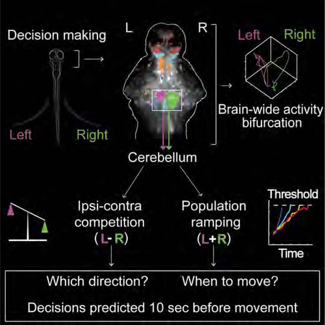
SUMMARY

Goal-directed behavior requires the interaction of multiple brain regions. How these regions and their interactions with brain-wide activity drive action selection is less understood. We have investigated this question by combining whole-brain volumetric calcium imaging using light-field microscopy and an operant-conditioning task in larval zebrafish. We find global, recurring dynamics of brain states to exhibit pre-motor bifurcations towards mutually exclusive decision outcomes. These dynamics arise from a distributed network displaying trial-by-trial functional connectivity changes, especially between cerebellum and habenula, which correlate with decision outcome. Within this network the cerebellum shows particularly strong and predictive pre-motor activity (>10 s before movement initiation), mainly within the granule cells. Turn directions are determined by the difference neuroactivity between the ipsilateral and contralateral hemispheres, while the rate of bi-hemispheric population ramping quantitatively predicts decision time on the trial-by-trial level. Our results highlight a cognitive role of the cerebellum and its importance in motor planning.

Graphical Abstract

In Brief:

A specific motor decision and its timing can be predicted using information from the cerebellum >10 seconds before movement, during a cognitive task in larval zebrafish. Decision outcomes and timing can be predicted at the single-trial level, using neuroactivity information from whole-brain Ca2+ imaging, at single-cell resolution.

INTRODUCTION

Animals interact with their environment in a goal-directed manner and through complex behaviors that are optimized over time. Such goal-directed behaviors require motor planning that precedes actions. The neuronal signatures of such preparatory activity have been reported in the motor (Churchland et al., 2010), pre-motor (Li et al., 2016) and parietal cortices (Maimon and Assad, 2006) and display a few common features (Gold and Shadlen, 2007; Murakami and Mainen, 2015; Shenoy et al., 2013; Svoboda and Li, 2018): First, preparatory activity can occur long before movement initiation. Examples include humans engaged in self-initiated binary decision tasks (Soon et al., 2008), mice during an instructed-delay task (Li et al., 2015), or primates involved in a visuomotor task (Maimon and Assad, 2006), for which preparatory activity encoding for decision outcomes several seconds preceding movement can be found in various cortical areas. Second, preparatory neuroactivity has been shown to manifest itself as a ramping or sequential activity to a threshold (Harvey et al., 2012) the rate of which has been shown to be correlated with decision timing (Gold and Shadlen, 2007; Maimon and Assad, 2006; Mazurek et al., 2003; Murakami and Mainen, 2015; Murakami et al., 2014; Wang, 2008; 2012). Finally, the neuroactivity of individual neurons during the pre-motor period can take more complex forms than merely a subthreshold version of movement-related activity (Churchland and Shenoy, 2007) and exhibit different tuning properties during different task epochs (Churchland et al., 2010). The common observation of variability in behavior (Gordus et al., 2015; Osborne et al., 2005) points towards dynamic trial-by-trial changes in the neurodynamics and thus cannot be captured by static and trial-averaged tuning frameworks for representation of motor responses (Afshar et al., 2011; Briggman et al., 2005; Churchland and Kiani, 2016; Wei et al., 2019).

While these findings in the cortex have provided insight, they also highlight the need for capturing neuronal population activity on a trial-by-trial basis and, as other studies have shown, for taking a brain-wide approach to decision making (Cisek and Kalaska, 2010; Gao et al., 2018; Guo et al., 2017; Horwitz and Newsome, 1999; Kunimatsu et al., 2018; Liu et al., 2013). Support for this notion comes from the fact that decision making requires access to or can be modulated by brain functions such as short-term memory, internal states and reward expectation that have a sub-cortical representation (Abbott et al., 2017; Allen et al., 2017). However, obtaining high spatiotemporal resolution access to whole-brain neuroactivity is currently not possible in mammalian brains, while studying complex goal-directed behaviors, motor planning and decision making in non-vertebrates is challenging and results may be not directly transferrable to vertebrates. The larval zebrafish represents an attractive model to investigate these questions due to its high level of physiological and genetic homology to the mammalian brain, conformity to basic vertebrate brain organization (Friedrich et al., 2010; Kalueff et al., 2014) and its transparent brain that allows for whole-brain in vivo optical recording of neuroactivity at high speed and cellular resolution utilizing recent techniques in two-photon (Ahrens et al., 2012; Portugues et al., 2014; Renninger and Orger, 2013), light field (Andalman et al., 2019; Cong et al., 2017; Nöbauer et al., 2017; Prevedel et al., 2014), light sheet (Ahrens et al., 2013; Favre-Bulle et al., 2018; Migault et al., 2018; Wan et al., 2019), and other forms of microscopy (Huisken et al., 2004; Wolf et al., 2015; Wu et al., 2011). However, establishing a robust behavioral paradigm in the larval zebrafish that involves learning, memory and integration of information across brain regions, and within which the neuronal basis of goal-directed motor planning and decision making could be studied, has proven challenging.

In the present study, we have combined high-speed volumetric calcium imaging based on light-field microscopy (LFM) (Nöbauer et al., 2017; Prevedel et al., 2014)—a technique that uniquely enables simultaneous capturing of neuronal network activity on the scale of the whole-brain at single-cell resolution—with a new operant conditioning paradigm in larval zebrafish, Relief Of Aversive Stimulus by Turn (ROAST, Li, 2013), to investigate the neuronal basis of goal-directed action selection. We found the dynamics of brain states to display decision-related bifurcation enabling prediction of both decision time and outcome at the trial-by-trial level. We found multiple brain areas whose inter- and intra-dynamics exhibited performance-dependent trial-by-trial changes of correlated pre-motor neuroactivity, representing functional connectivity changes which cannot be explained by slower learning-based changes of the network. The cerebellum also exhibited a surprisingly strong level of preparatory neuroactivity, which we found to mainly originate from the granule cell population, and which allowed us to predict both turn direction and the timepoint of turn initiation ~10 seconds before movement for individual trials. Our observations are explained by a model in which turn direction is determined by cerebellar ipsi-contralateral competition, while the timepoint of turn initiation is quantitatively predicted by the joint ipsi-contralateral population ramping rate.

Thus, our work extends the traditional view of the cerebellum in motor control and provides support for its more cognitive functions, while expanding the existing frameworks of “ramping-to-threshold” for decision making (Gold and Shadlen, 2007; Wang, 2012) to the level of individual trials which has not been possible due to technical limitations (Shadlen et al., 2016). The presence of cerebellar preparatory activity, representing internal variables that cannot be directly explained by instantaneous behavior or sensory input, points towards the critical role that it could play in motor planning more generally and, as zebrafish lack a cortex, prior to the emergence of cortical regions and functions (Hodos, 2009).

RESULTS

An operant conditioning paradigm for larval zebrafish

In ROAST, fish learn to perform a directed tail movement to the right or left in order to receive relief from an aversive heat stimulus (Figure 1A). While ROAST was initially developed to study learning (Li, 2013), it also provides an ideal opportunity to investigate the neuronal basis of action selection and underlying pre-motor activity. The binary nature of the decision as well as the extended decision time (DT), between the onset of heat stimulus and the initiation of the first movement, allow studying the neuronal dynamics that underlie the choice for turn direction as well as the timing of movement initiation (see STAR Methods). Data from an example learner is shown in Figure 1B. The learners’ performance typically became stable after the first 15 trials in both blocks, with an asymptotic final performance of ~80% correct (Figure 1C, see STAR Methods). At the level of single trials, we found that the latency to heat offset decreased as a function of trials in learner fish (Figure S1A) while the mean DT remained stable (Figure S1B). We performed simultaneous whole-brain calcium imaging using a home-built LFM (Nöbauer et al., 2017; Prevedel et al., 2014) and a transgenic fish line Tg(elavl3:H2B-GCaMP6s) (Vladimirov et al., 2014) while animals were engaged in ROAST. Using LFM allowed us to capture cellular neuroactivity at the whole-brain level within a volume of 700×700×200 μm, with all voxels acquired truly simultaneously at a volume rate of 10 Hz.

Figure 1. An operant conditioning assay for larval zebrafish combined with whole-brain calcium imaging.

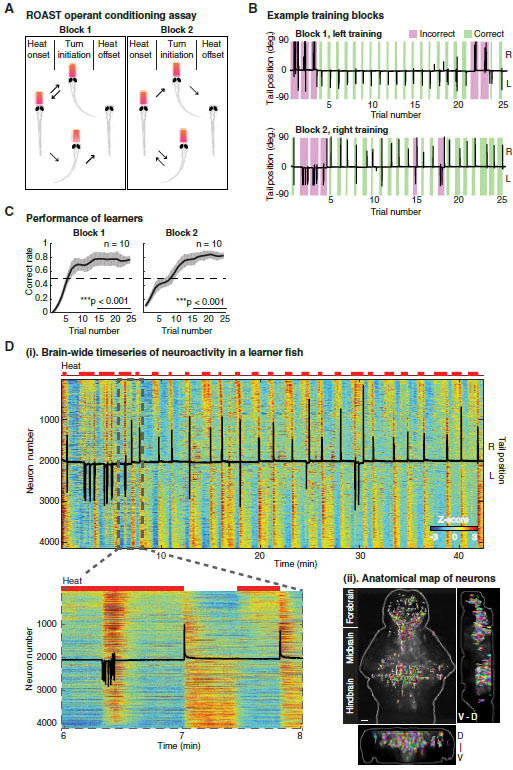
(A) Relief of Aversive Stimulus by Turn (ROAST). Head-fixed larval zebrafish receive a mildly aversive heat stimulus by an infrared laser (red trapezoid) at the beginning of a trial. The laser is turned off if the fish makes a tail movement in the reward direction and remains on otherwise. In the second training block the reward direction is switched, with each block consisting of 20–25 trials (see STAR Methods).

(B) The learning progress (two blocks) of an example learner (8 dpf). Black traces indicate tail positions over time, magenta and green rectangles indicate the duration of the heat stimulus for each incorrect and correct trial, respectively.

(C) Averaged performance as a function of trial number (mean ± SEM, n = 10). The correct rate in the first 10 trials is significantly below 0.5, **p = 0.001 for block 1 and *p = 0.012 for block 2; the correct rate in the last 10 trials is significantly above 0.5, ***p < 0.001 for both blocks (bootstrapping, n = 5000).

(D) (i) Heat map of brain-wide neuronal time series (Z-scored) from a learner with top 2% most active voxels extracted and segmented, resulting in 4124 neurons. Neurons sorted by their correlations with heat stimuli, from highly positive to highly negative. Upper red bars: heat stimuli; superimposed black trace: tail position of the fish; lower panel: zoom into the dashed rectangular area.

(ii) Anatomical map of same extracted neurons as in (i), displayed in random colors for clarity. Scale bar, 50 μm.

Recurring brain state dynamics show bifurcation for different decision outcomes

Volumetric reconstruction of the LFM data (see Movie S1), followed by neuronal signal extraction (Prevedel et al., 2014), allowed us to obtain activity traces from ~5,000 of the most active neurons across the brain (Figure 1D, example learner in Block 2, right training). When these activities were co-registered with the time period of heat stimulus and the timepoints of left or right tail movements, a significant level of correlation was observed (Figure 1D (i)). Mapping these neuronal activities spatially onto the brain revealed active neurons across the entire forebrain, midbrain and anterior hindbrain (Figure 1D (ii)), which were consistent in number and distribution across specimens (Figure S1D,E) with distinct neuronal dynamics in different brain regions correlated with specific epochs of our task (Figure S1C). To identify how the dynamics of brain states—i.e., the state of activity of all neurons at a given time—are associated with the different task epochs, we began by performing linear dimensionality reduction based on principal component analysis (PCA). However, PCA on brain states failed to effectively reduce dimensionality in a fashion that would capture key differences during different task epochs (Figure S1F,G). To overcome this issue, we applied a nonlinear dimensionality reduction technique, t-distributed stochastic neighbor embedding (t-SNE, see STAR Methods), to the time series of brain states (Maaten and Hinton, 2008).

We found two major clusters that were associated with the presence and absence of the heat stimulus, respectively (Figure S2A), showing that changes of the heat stimulus drive temporally sharp transitions between brain states resulting in a higher similarity of intra-cluster brain states than inter-cluster brain states (Figure S2B). Investigating the brain state representation of decision-related behavior, we found that brain states corresponding to correct and incorrect turns each densely and distinctively occupied separate sub-regions of the “Heat ON” and “Heat OFF” clusters (Figure 2A) with an increased level of similarity of brain states before turn events, in particular for correct trials (Figure S2C,D). These observations show stereotypical, reoccurring global brain states across trials with increased coordination before movement, particularly in correct trials.

Figure 2. Decision making relies on coordination and integration of distributed information across the whole brain.

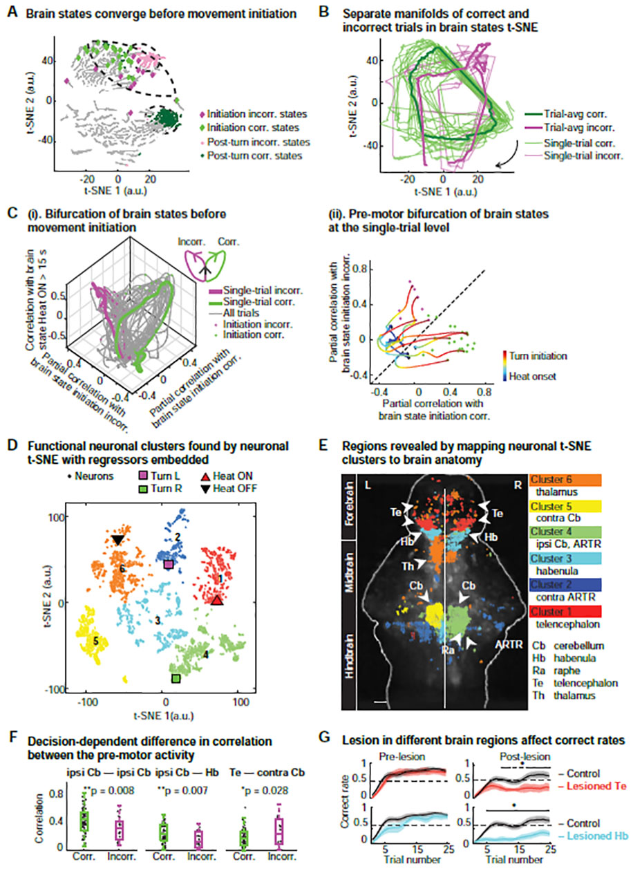
(A) Brain states for a given trial type (correct or incorrect) converge into a smaller region of the t-SNE space before turn initiation (diamonds; incorrect (incorr.): magenta, correct (corr.): green) and are well-separated post turn, i.e. 0–10 s after movement initiation (circles; incorrect: magenta, correct: green). See also Figure S2C,D.

(B) Temporal evolution of brain states during correct versus incorrect trials lie on separate cyclic manifolds, visualized in a 2D map; single trials (thin lines) and trial averages (thick lines); arrow: direction of temporal evolution. Manifold separation measured with Hausdorff distance (Bruno et al., 2017), ***p < 0.0001, Wilcoxon rank sum test.

(C) Performance-dependent bifurcation of brain states before turn initiation. See STAR Methods.

(i) After heat onset, brain states exhibit similarity along the “Heat ON” dimension (vertical axis), followed by a pre-turn bifurcation towards the correct or incorrect state. Similarity is measured by partial correlation between a given brain state and the average correct, incorrect or “Heat ON” state.

(ii) 2D representation of single-trial bifurcation process. Individual correct and incorrect trials are highlighted during the pre-motor period (Black diamonds: heat onset, green and magenta dots: turn initiations for correct and incorrect turns, respectively). See also Movie S2.

(D) Application of t-SNE on neuron space reveals six distinct functional clusters of neurons (different colored circles) with behavior and stimulus regressors embedded in a 2D t-SNE map (triangles and squares). The t-SNE map is partitioned by hierarchical clustering (see STAR Methods). The “Heat ON” regressor (red triangle) is located in Cluster 1, “Heat OFF” in Cluster 6 (black triangle), “Turn R” in Cluster 4 (green square) and “Turn L” in Cluster 2 (magenta square).

(E) Mapping of functional neuronal t-SNE clusters onto brain anatomy reveals distinct overlap with specific anatomical regions. Cluster 1 is mainly in the telencephalon (Te); Cluster 2 in the left hindbrain contains “Turn L” regressor and overlaps with the left ARTR; Cluster 3 overlaps with the habenula (Hb) and the raphe (Ra); Cluster 4 contains “Turn R” regressor and overlaps with right (ipsilateral) cerebellum (Cb) and ARTR; Cluster 5 overlaps with the left (contralateral) cerebellum (Cb); Cluster 6 overlaps mainly with thalamus (Th) and parts of the Te and contains the “Heat OFF” regressor. Scale bar, 50 μm.

(F) Performance-dependent trial-by-trial changes in correlation between pre-motor neuroactivity across brain regions. The absolute correlation of activity within the ipsilateral cerebellum (ipsi Cb) and between the ipsi Cb and other brain regions (Hb) increases in correct trials (green circle) compared to incorrect trials (magenta circle). Between other brain regions (e.g. between Te and contra Cb), correct trials exhibit a lower degree of correlation than incorrect trials. In particular, the difference in correlation between the ipsi Cb and Hb for correct versus incorrect trials is highly significant. Two-tailed t-test, *p < 0.05, **p<0.01. See also Figure S2F.

(G) Lesions in the habenula and telencephalon affect the correct rate and learning. Larvae that were lesioned in the Hb or Te exhibited a significant decrease in correct rate post-lesion compared to unlesioned larvae. n = 15 for the control group without lesion; n = 9 for the Te lesion group; n = 10 for the Hb lesion group. Wilcoxon rank sum test, one-tailed.

We connected temporally consecutive brain states in the t-SNE map on the trial-by-trial level and found the brain state dynamics to form a cyclic manifold, with the correct and incorrect trials forming distinct loops (***p < 0.0001, Wilcoxon rank sum test, Figure 2B). This shows that during correct trials, highly similar brain states occur across trials, despite the different duration of the stimulus in each trial and the different timing of the decisions. Projecting the brain states into a 3D space spanned by reference brain states for correct trials, incorrect trials and the heat-encoding component (see STAR Methods) revealed a clear pre-turn bifurcation (Figure 2C) towards the correct and incorrect decision state. Strikingly, the bifurcation towards different decision outcomes could be observed well before turn initiations at the single-trial level (Figure 2C (ii), Movie S2), despite different DTs.

Performance-dependent brain-wide changes in functional connectivity precede motor response

Given our observations at the level of brain states, we set out to investigate the brain regions that drive the bifurcation towards different decision outcomes. We applied t-SNE to each neuron’s activity patterns in order to partition them into functional neuronal clusters. Applying t-SNE to the time series of all neurons and that of four behavior and stimulus regressors (Figure S2E, see STAR Methods) allowed us to identify the individual functional neurons and their clustering around our regressors, which we emphasized further by partitioning the t-SNE map using hierarchical clustering (see STAR Methods). Using this approach, six neuronal clusters with four regressors embedded within them were found (Figure 2D). We found that the t-SNE clusters coincided well with distinct anatomical regions (Figure 2E). A distinct group of bilateral neurons (Cluster 1) in the telencephalon (Te) responded to the onset of the heat stimulus, “Heat ON”. Another group (Cluster 6), overlapping largely with the thalamus, but also with neurons sparsely distributed in the Te, encoded for “Heat OFF”. “Turn L” was represented by contralaterally located neurons in the hindbrain and the left adjacent anterior rhombencephalic turning region (ARTR, Cluster 2) (Dunn et al., 2016; Wolf et al., 2017), while “Turn R” was encoded by neurons in the ipsilateral right hindbrain that highly overlapped with the cerebellum and ARTR and fell into a single cluster (Cluster 4). Cluster 3 overlapped with habenula and raphe, while Cluster 5 coincided with the left cerebellum.

We hypothesized that decision making underlying goal-directed behavior relies on the coordination and integration of distributed information across different brain regions. While this notion has been theoretically proposed (Abbott et al., 2017; Svoboda and Li, 2018), to our knowledge it has not been directly demonstrated experimentally. To investigate this, we used correlation (Cohen and Kohn, 2011; Kohn et al., 2016), and evaluated it at the single-trial level for the relevant functional neuronal clusters for correct versus incorrect trials (Figure 2F, S2F). We found that the absolute correlation of pre-motor activity within the ipsilateral cerebellum (ipsi Cb), as well as between the ipsi Cb and other brain regions such as the habenula (Hb) and the contralateral cerebellum (contra Cb), increase on a trial-by-trial level, with correct trials exhibiting a higher degree of correlation than incorrect trials (Figure S2F). In particular, we found the average difference in correlation of pre-motor neuroactivity between the ipsi Cb and Hb for correct versus incorrect trials to be highly significant (Figure 2F). Moreover, we show that these trial-by-trial changes of correlation, which represent changes of functional connectivity, cannot be explained by the direct training-related changes of the network as the ipsi Cb and Hb did not show a significant change in their correlated activity as a function of training (Figure S2F). In order to establish that the observed coordination and integration of brain-wide signals are necessary for correct decision outcomes, we performed pre-training lesions in Te and Hb. We found that both lesions impair the fish’s ability to learn and make correct decisions (Figure 2G). These observations strongly support the notion of a necessary integration and coordination of information across and within brain regions to generate motor planning for correct decision outcomes.

We next searched for the neuroactivity within each cluster that contributed to the observed pre-motor bifurcation of brain states and thus would be predictive of the motor response. However, since neurons can in principle have a mixed response, i.e. also decision-independent components such as those associated with the stimulus, it was necessary to parse out the decision-dependent versus decision-independent components from each cluster. To do so, we used demixed principal component analysis (dPCA, Kobak et al., 2016, see STAR Methods, Figure S3A,B). We found the dPC1 of all clusters to account for at least ~50% of the observed variance in the corresponding cluster, and to exhibit a decision-independent response (Figure 3A). Consistent with our observation of the t-SNE map where the “Heat ON” regressor is embedded in Cluster 1 (Te), we found the dPC1 of Cluster 1 to show increased activity only after heat onset. dPC1 of Cluster 2 (contra ARTR) showed increased activity only after turn initiation, suggesting it is encoding for movements, while dPC1 of Clusters 3 (Hb) and 4 (ipsi Cb and ARTR) displayed a linear increase in activity upon heat onset followed by a secondary peak after turn initiation, suggesting their potential involvement in sensorimotor transformation. dPC1 of Clusters 5 (contra Cb) and 6 (thalamus) showed an overall decreased activity upon heat onset—in contrast to the neuroactivity in Clusters 4 and 1, respectively—followed by an increase of activity after turn initiation. dPC2 explained ~25% of observed variance in each cluster. Importantly, we found that it exhibited in all clusters a decision-dependent behavior with a clear separation of correct versus incorrect decisions, in some clusters prior to and in some clusters after initiation of motor behavior (Figure 3A, see STAR Methods). Among these clusters, Cluster 4, the ipsi Cb and ARTR, allowed for a reliable decoding of the turn direction well before turn initiation. Overall, even though the pre-motor signal is available across multiple brain areas, the cerebellum and ARTR contain the strongest predictive signal for decision direction.

Figure 3. Preparatory activity in the cerebellum is highly predictive of decision outcome and emerges through training.

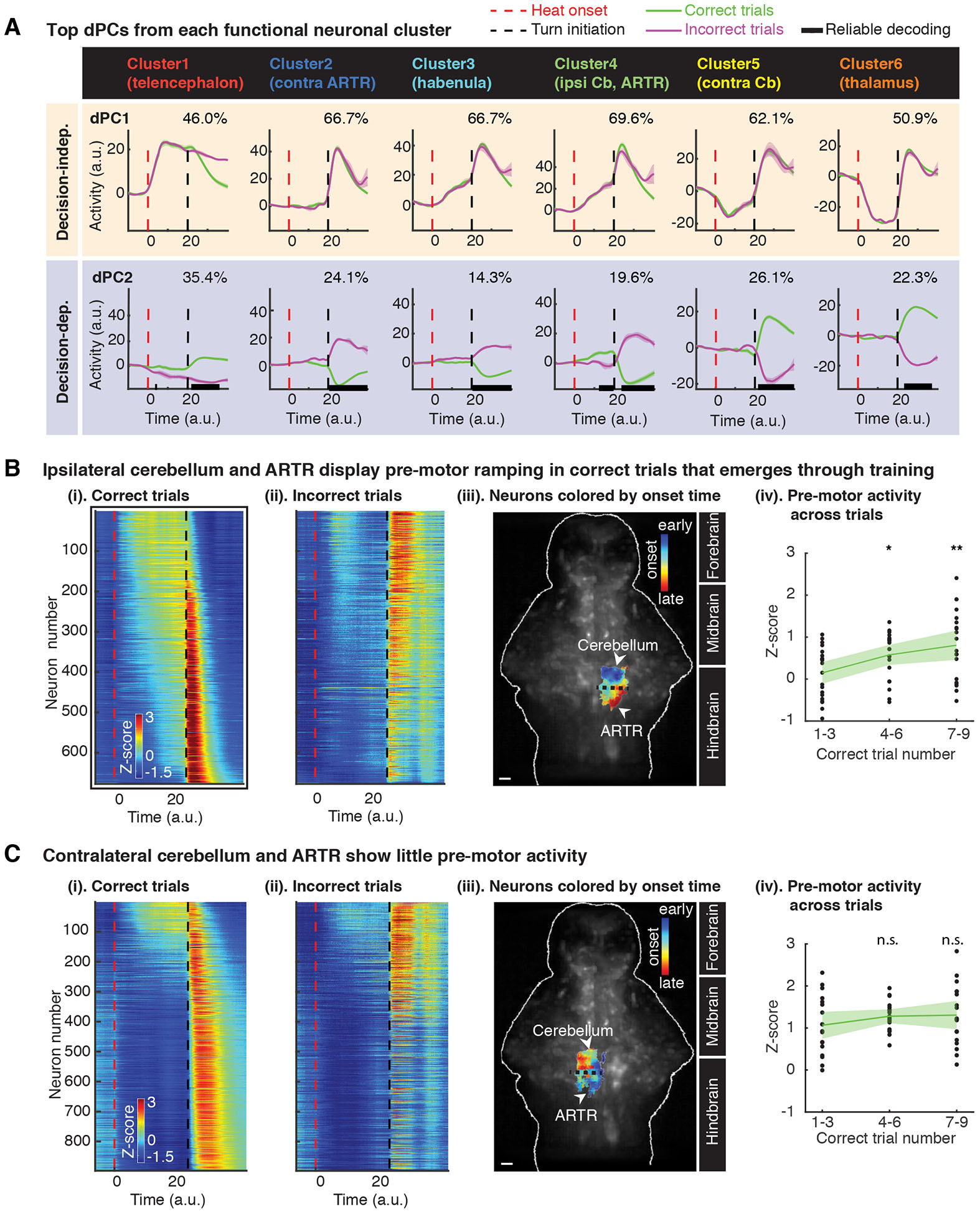
(A) Top demixed principal components (dPCs) from each functional neuronal cluster. Population activity from each cluster was projected onto individual dPCs and averaged over trials (lines and shaded bands: mean ± 1.96 SEM). Explained variance for each dPC is given at the top right of each panel. Horizontal black bars on x-axis mark timepoints when correct versus incorrect trials can be reliably decoded (see STAR Methods). Pre-motor decision-dependent signal (in which the time of decoding precedes and lasts until turn initiation time) is observed from dPC2 of Cluster 4, the ipsi Cb and ARTR. Post-turn decoding is reliably possible from the dPC2 of all functional clusters, but only Cluster 4 allows for reliable pre-motor decoding. Time series were processed for co-alignment from heat onset to turn initiation, i.e. the decision time (see STAR Methods).

(B) Ipsilateral cerebellum and ARTR display strong pre-motor ramping activity in correct trials that emerges through training.

(i) & (ii). Pre-motor activity of individual neurons in ipsi Cb and ARTR averaged over correct or incorrect trials. Neurons in both panels are sorted according to onset timing of pre-motor activity during correct trials. Red dashed lines, heat onset; black dashed lines, turn initiation.

(iii). Anatomical locations of ipsilateral neurons color-coded according to the onset time of their pre-motor activity. Onset time of activity increases from anterior (Cb) to posterior (ARTR) in the ipsilateral hindbrain. Background: anatomical reference. Scale bar: 50 μm.

(iv). Pre-motor activity, averaged from individual neurons, significantly increases with training. Each dot represents pre-motor activity from a single trial. Trials are combined across 7 datasets. *p < 0.05, **p < 0.01, ***p < 0.001, two-tailed Wilcoxon rank sum test.

(C) Contralateral cerebellum and ARTR show little pre-motor activity.

(i) & (ii). Pre-motor neuroactivity of individual neurons in contra Cb and ARTR averaged over correct or incorrect trials. Neurons in both panels are sorted according to the onset time of pre-motor activity during correct trials.

(iii). Anatomical distribution of contralateral neurons, which are color-coded according to the onset time of their pre-motor activity. Onset time of activity increases from posterior (ARTR) to anterior (Cb) in the contralateral hindbrain. Background: anatomical reference. Scale bar, 50 μm.

(iv). Preparatory activity, averaged from individual neurons, shows no significant change as training progresses. Each dot represents pre-motor activity from one trial. Trials are combined across the same animals as in B. Two-tailed Wilcoxon rank sum test.

Cerebellar ipsi-contralateral difference neuroactivity predicts decision outcome on the trial-by-trial level

Given our above observations on the pre-motor decision-dependent dPCs of the cerebellum and ARTR, we hypothesized that they may represent preparatory neuroactivity for motor planning, similar to what has been reported in the cortex (Churchland et al., 2012; Gao et al., 2018; Li et al., 2016). We first looked at the trial-averaged activity of individual neurons in Cluster 4, the ipsi Cb and ARTR. For correct trials, we observed a gradual increase of ipsi neuroactivity after heat onset which continued until movement initiation, followed by a strong peak after the execution of the turn (Figure 3B (i)). In contrast, for incorrect trials, neuroactivity was reduced in general. In particular, the above gradual increase of pre-motor neuroactivity was absent, although the post-turn peak remained present (Figure 3B (ii)). Sorting neurons both within correct and incorrect trials according to their activity onset time in the correct trials, we found that the identity of neurons that displayed strong activity after turns was different in correct versus incorrect trials (Figure 3B (i–ii)). Moreover, neurons that displayed strong post-turn activity in incorrect trials were the same ones that also showed early onset of strong pre-motor activity in correct trials (Figure 3B (i–ii)). This indicates that individual neurons displayed different ‘tunings’ during pre-motor and post-motor epochs of the task, and that pre-motor neuroactivity was not merely a subthreshold version of motor response (Churchland et al., 2010). We then mapped the order by which neurons became active to their anatomical locations in the brain. Following an anterior to posterior gradient, we found that neurons with an earlier onset time of pre-motor activity were located in the cerebellum while neurons with a later onset of activity were mainly located in the ARTR (Figure 3B (iii)). To exclude the possibility that the observed pre-motor activity represents an innate feature of the cerebellum, we investigated its changes as a function of trials. We found that the observed pre-motor activity uniquely emerges through learning in the ipsilateral side (Figure 3B (iv)) for correct trials. This observation also highlights the fact that a more complex behavioral task is indeed necessary to observe the cerebellar ramping activity. Compared to the ipsilateral side, the contralateral side displayed very little pre-motor ramping. In correct trials, the responses of the first few active neurons were similar to those of the ipsilateral side, however significantly fewer neurons participated in the pre-motor ramping activity, while a similarly strong post-turn response persisted for the correct trials (Figure 3C (i)). In incorrect trials, neurons that displayed strong post-turn activity had an early onset time of pre-motor activity (Figure 3C (ii)), and mostly overlapped with the contra ARTR (Figure 3C (iii)). Consistent with our above observation of weak ramping activity in the contra Cb, we found no significant changes in contralateral ramping activity as a function of trial in our learning task (Figure 3C (iv)).

The ARTR in each hemisphere has been shown to project inhibitory connections to the contralateral hemisphere (Dunn et al., 2016). Moreover, the parallel fibers of the cerebellar granular neurons, which feed into the Purkinje cells, span across both hemispheres of the cerebellum densely (Knogler et al., 2017). These observations provide evidence that the contra ARTR and Cb are an integral part of the learning, motor planning and action selection circuit and that the activity of the ipsi and contra ARTR and cerebellum should be analyzed collectively. Thus, we investigated the joint dynamics of Clusters 2, 4 and 5 during different task epochs, decomposed their joint activity into decision-independent and decision-dependent activity by applying dPCA, and focused on the top 4 dPCs, which explain >80% of the variance. Within the decision-independent components, dPC1 displayed ramping and dPC3 a plateau, while for the decision-dependent components, dPC2 exhibited post-motor separation and dPC4 pre-motor separation (Figure 4A, S4A). The observed ramping mode of dPC1 is consistent with activity that would represent a non-direction-specific, but rather temporal aspect of a decision (i.e., the DT), while the plateau region in dPC3 is consistent with heat-and-motor-evoked signals, as the rise and fall of dPC3 coincides with heat onset and movement initiation. dPC2 represents the decision outcome after the turn—which can serve as a feedback signal for learning—while dPC4 represents the feed-forward pre-motor signal that encodes future turn direction. In both non-learners (Figure S4B) and fish performing spontaneous turns in the absence of a heat stimulus (Figure S4C), the post-motor feedback signals were present, but pre-motor cerebellar signals were not predictive of turn direction.

Figure 4. Bilateral ipsi-contra competition in the cerebellum determines decision outcome.

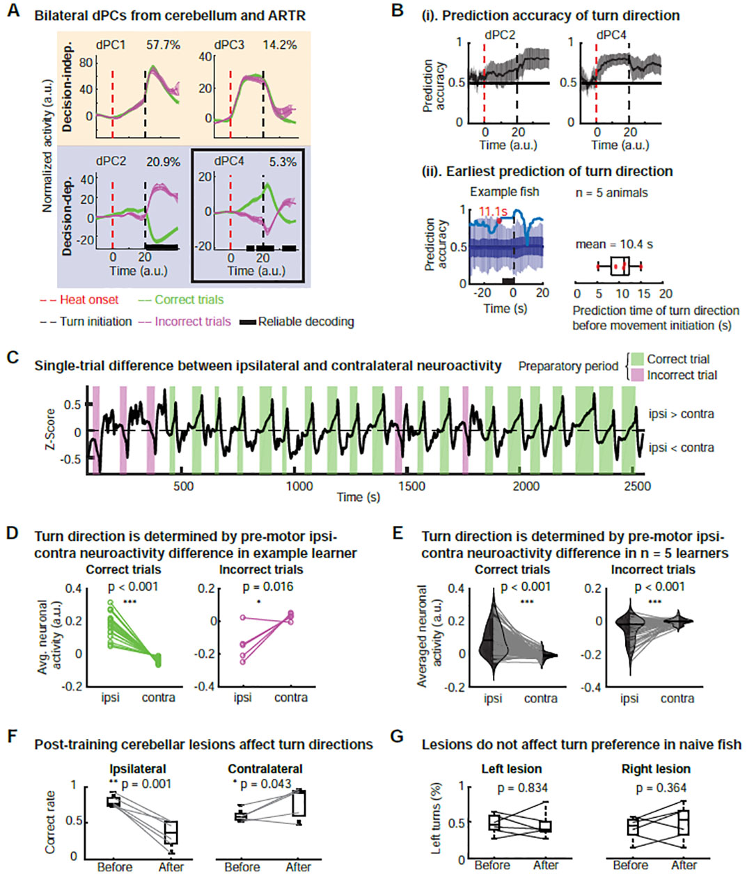
(A) Bilateral dPCA analysis of joint neuroactivity of cerebellum (Cluster 4 and Cluster 5). Decision-independent dPCs: dPC1 displays pre-motor ramping and post-turn peak; dPC3 displays a plateau shape for most of the decision time, representing the heat- and motor-evoked signals. Decision-dependent dPCs: dPC2 shows post-turn separation, which could serve as a feedback signal; dPC4 displays pre-motor separation, the signal to plan and drive action selection. Data from a representative fish.

(B) Decision direction can be predicted as early as 10 seconds before movement initiation with an average accuracy of 80%.

(i) Prediction accuracy for correct versus incorrect turns extracted from decision-dependent dPCs. dPC2 displays post-turn classification of correct versus incorrect trials while dPC4 allows for pre-turn prediction of turn direction, with an average accuracy as high as 80%. Prediction accuracy from n = 8 training blocks of 5 learners, mean ± 1.96 SEM.

(ii) The prediction timepoint (red dot) in an example learner. Dark blue line and shaded band: mean and SD of shuffling tests (n = 100). See STAR Methods and Figure S3D.

(iii) Earliest prediction times from 7 learner datasets, in 5 of which prediction precedes movement initiation (mean prediction time: 10.4 s).

(C) Pre-motor difference neuroactivity between the ipsi and contra Cb as a function of time. Data are constructed from the pre-motor decision-dependent activity from an example learner (see Figure S4D).

(D) Trial-by-trial comparison of pre-motor neuroactivity between ipsi and contra sides for correct versus incorrect trials of an example learner. Wilcoxon signed rank test, one-tailed. See STAR methods.

(E) Trial-by-trial comparison of pre-motor neuroactivity between ipsi and contra sides for correct versus incorrect trials. Data pooled across 5 learners, with 144 correct trials and 56 incorrect trials. Wilcoxon signed rank test, one-tailed.

(F) Post-training lesions in the cerebellum affect the distribution of turn directions. Laser-induced lesions in the ipsi Cb (n = 6) result in a significant decrease of the correct rate, while lesions in the contra Cb result in a mild increase of the correct rate (see discussion, n = 5). Each gray line represents one two-block learner animal. Only trials with behavioral responses are used for calculating the correct rate. One-tailed t-test.

(G) Lesions in naïve animals do not affect the distribution of turn directions. The fraction of left turns before and after lesion was counted in freely behaving zebrafish without exposure to any heat stimulus. n = 6 for lesions in each side, two-tailed t-test.

Next, given our observations on the pre-motor decision-dependent dPCs in learners, we set out to quantify how well these predicted the outcome of the turn before movement initiation at the trial-by-trial level. Our prediction accuracy analyzed across fish (see STAR Methods, n = 8 training blocks) reached ~80% before turn initiation (Figure 4B (i)). Figure 4B (ii) shows the prediction time in our example learner dataset, for which we found a value of 11.1 s (see STAR Methods and Figure S3C,D). This result was reproducible across multiple learners (n = 5) for which we found an average prediction time of 10.4 s (Figure 4B (ii)). The above time scales are different from the millisecond time scale that has been traditionally associated with the role of the cerebellum in motor control (Johansson et al., 2016), but well within the range of working memory (Buhusi and Meck, 2005; Tetzlaff et al., 2012).

We speculated that the decision for turn direction might arise from an ipsi-contra interaction between the neuroactivity in the cerebellum, with the “winning” side determining the decision outcome. We tested this idea by comparing the difference in the decision-dependent neuroactivity of the Cb and ARTR between the two hemispheres during the pre-motor period at the single-trial level (see STAR Methods). Compared to the original neuronal time series, this reconstructed time series only contained pre-motor decision-dependent information but had the same dimension (i.e. neurons × time, Figure S4D). Thereby, we could preserve the information on the location of each neuron and obtain the ipsi-contra difference activity. An example of the ipsi-contra difference of reconstructed neuroactivity as a function of time is shown in the Figure 4C, where it is positive during correct trials and negative during incorrect trials.

For an individual learner, we found a significantly higher level of preparatory activity on the ipsilateral side than the contralateral side in correct trials, but a significantly lower level of activity in the incorrect trials (Figure 4D). These observations were consistent across fish and when all trials were pooled (Figure 4E), but not present in non-learners (Figure S4E,F). This mirroring relationship between the ipsilateral and contralateral side was seen in dPC4 across animals, but none of the other three top dPCs. Post-training ipsi Cb lesions led to a significant decrease in the correct rate, whereas contra Cb lesions resulted in a slight increase in the correct rate (Figure 4F). In fish performing spontaneous turns without stimuli, cerebellar lesions did not affect turning preference (Figure 4G), consistent with our previous observations that pre-motor cerebellar is only present in fish that learned (Figure S4A–C). These observations support our idea that cross-hemisphere difference neuroactivity in the cerebellum during motor planning forms the basis of the decision for turn direction, with the more active side determining the decision outcome on the trial-by-trial level.

The ramping rate of bilateral cerebellar population dynamics determines decision time at the trial-by-trial level

A number of previous studies have shown that in various decision-making tasks, the DT is linked to the velocity of the increase of cortical preparatory activity (Afshar et al., 2011; Hanes and Schall, 1996; Murakami et al., 2014; Shenoy et al., 2013; Wang, 2012). Given our observation of ramping in the decision-independent pre-motor component of the cerebellar neuroactivity (Figure 4A, dPC1), we asked if the rate of this ramping would be correlated with DT at the trial-by-trial level. We found trials with a shorter DT to exhibit a higher ramping rate and those with a longer DT a lower ramping rate (Figure 5A). We then calculated the ramping rate by a linear fit of the population activity (Z-score of dPC1) from heat onset to one second before the turn (Figure S5A) and found the ramping rate to be linearly correlated with the logarithm of the DT at the single-trial level (Figure 5B). We further confirmed that such an inverse correlation exists across animals at the single-trial level, despite systematic differences in the average DT of each fish (Figure 5C).

Figure 5. Bilateral cooperation of cerebellar neuroactivity determines decision time.

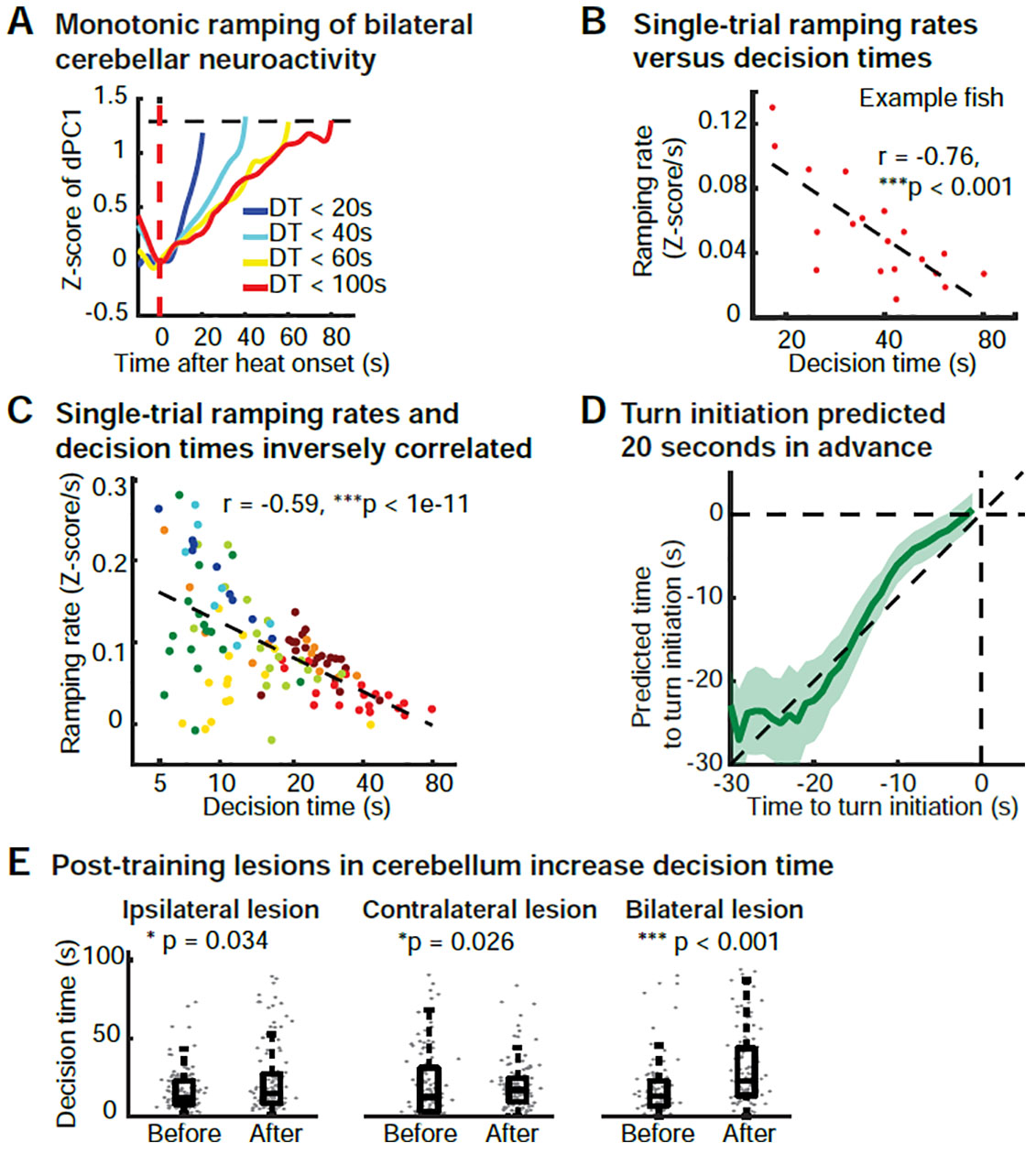
(A) Monotonic ramping of bilateral cerebellar population activity grouped by decision time (DT). Turns appear to be initiated when ramping activity reaches a common decision-time-independent threshold. Population activity (dPC1) is grouped in 4 categories of DTs and then averaged across trials. Each trace is from the heat onset (red dashed line) to the initiation of the first turn. Black dashed line indicates arbitrarily chosen threshold. Data from a representative learner.

(B) Ramping rate of population dynamics (dPC1) as a function of the DT at the single-trial level. Ramping rate is calculated by linear fit of pre-motor ramping activity (from heat onset to 1 s before turn initiation, see Figure S5A). Data points are single trials from a representative learner.

(C) Bilateral cerebellar ramping rate of population activity is inversely correlated with the DT at the single-trial level across multiple animals. 114 trials from 8 training blocks are shown in different colors from 5 animals.

(D) The accuracy of the prediction time of the movement initiation versus time. The accuracy of the prediction time of movement initiations increases with time after heat onset and approaches the actual movement initiation time ~20 seconds before turn initiation (22.3 s ± 2.5 s when t = 20 s, mean ± SEM). Single-trial predicted values (mean ± 1.96 SEM, see also Figure S5B) from 5 fish are plotted against actual values.

(E) Post-training cerebellar lesions increase DT. One-tailed Wilcoxon rank sum test, n = 6 for ipsi Cb lesions, 5 for contra Cb lesions, and 7 for bilateral lesions.

Next, we asked if the population ramping rate is predictive of the time of turn initiations on the single-trial level. We obtained the fit parameters for a linear ramping and used this linear model to make a prediction about the expected turn initiation time at any given timepoint t after the heat onset (Figure S5B, see STAR methods). As expected, we found the predicted turn initiation time to become more accurate as t approached the turn initiation timepoint and to be highly predictive for actual turning time within a 20-second window before the turn (22.3 s ± 2.5 s when t = 20 s, mean ± SEM), at the single-trial level (Figure 5D, Movie S3). To provide further causal support for our proposed mechanism, we performed both unilateral and bi-lateral post-training cerebellar lesion experiments. We found that, consistent with our model, both types of lesions, performed independently or together, led to a general increase of the DT (Figure 5E) as they reduced the pool of neurons contributing to the bi-hemispheric ramping signal.

In principle, such ramping could be facilitated by a gradual increase of activity in individual neurons, which seemed unlikely due to their various complex forms at single-trial level (Figure S5C), or from more neurons joining the population of active neurons over time and participating in the generation of ramping activity on a population level. We found a high level of similarity between the ramping activity (dPC1) and the degree of neuronal participation (r = 0.799, ***p < 0.0001, see STAR methods), while the observed correlation of single-neuron activities with the population ramping activity was lower and ~82% of all neurons showed a lower degree of correlation with the population ramping activity compared to the degree of neuronal participation (Figure S5D). This suggests that an increase in the number of active neurons is more likely to be the source of observed ramping activity than a gradual increase in activity in individual neurons. The remaining 18% of neurons overlapped with the ipsilateral ARTR (Figure S5E).

We next aimed to determine which of the main cerebellar cell types, namely the Purkinje, granule and eurydendroid cells, were the primary contributors to cerebellar ramping activity. We used Tg(gSA2AzGFF152B; UAS:GCaMP6s) (Filosa et al., 2016; Knogler et al., 2017; Takeuchi et al., 2015) which specifically labels the granule cells with GCaMP and allowed us to separate the contribution of granule cells and the cerebellar output neurons. We found the granule cells to display strong pre-motor activity (Figure 6A (i)). To differentiate between the activity of the Purkinje and eurydendroid cells, which are intermingled in the zebrafish cerebellum (Bae et al., 2009; Takeuchi et al., 2015), we utilized Tg(Huc:H2B-GCaMP6s; GAD1b:RFP) (Freeman et al., 2014; Satou et al., 2013) in which the Purkinje cells are most strongly labeled in GAD1b:RFP (Bae et al., 2009). We took advantage of the anatomy and the fact that the Purkinje cells in fish are predominately located in dorsal layer of the cerebellum (Bae et al., 2009; Takeuchi et al., 2015). We found pre-motor activity, although at different levels, for all three cell types (Figure 6A (i–iii)). Individual neurons exhibited a response that was either positively or negatively tuned to the decision outcome. We found that more than 70% of recorded neurons of these three cell types displayed significant differences in pre-motor activity in correct compared to the incorrect trials. This could be also clearly observed for the Purkinje cell population, despite its overall lower level of premotor activity (Figure 6A (ii)), suggesting that our observed pre-motor turn direction prediction is driven by the neuroactivity of a large, diverse cerebellar population. Given that the eurydendroid cells are known to integrate input from both the granule and Purkinje cells (Figure 6A (iv)), our data suggest that the main source of the observed pre-motor ramping activity predictive of the DT is stemming mainly from the granule cells rather than the Purkinje neurons. However, we observe a significant increase in post-turn activity in the Purkinje cells (p < 0.05) in incorrect trials that may represent feedback via the climbing fibers. This observation is also consistent with recent mammalian studies show that the granule cells represent learning and reward-related signals (Giovannucci et al., 2017; Wagner et al., 2019; 2017).

Figure 6. Proposed model for decision-making network in cerebellum, and the interaction with brain-wide neurodynamics.

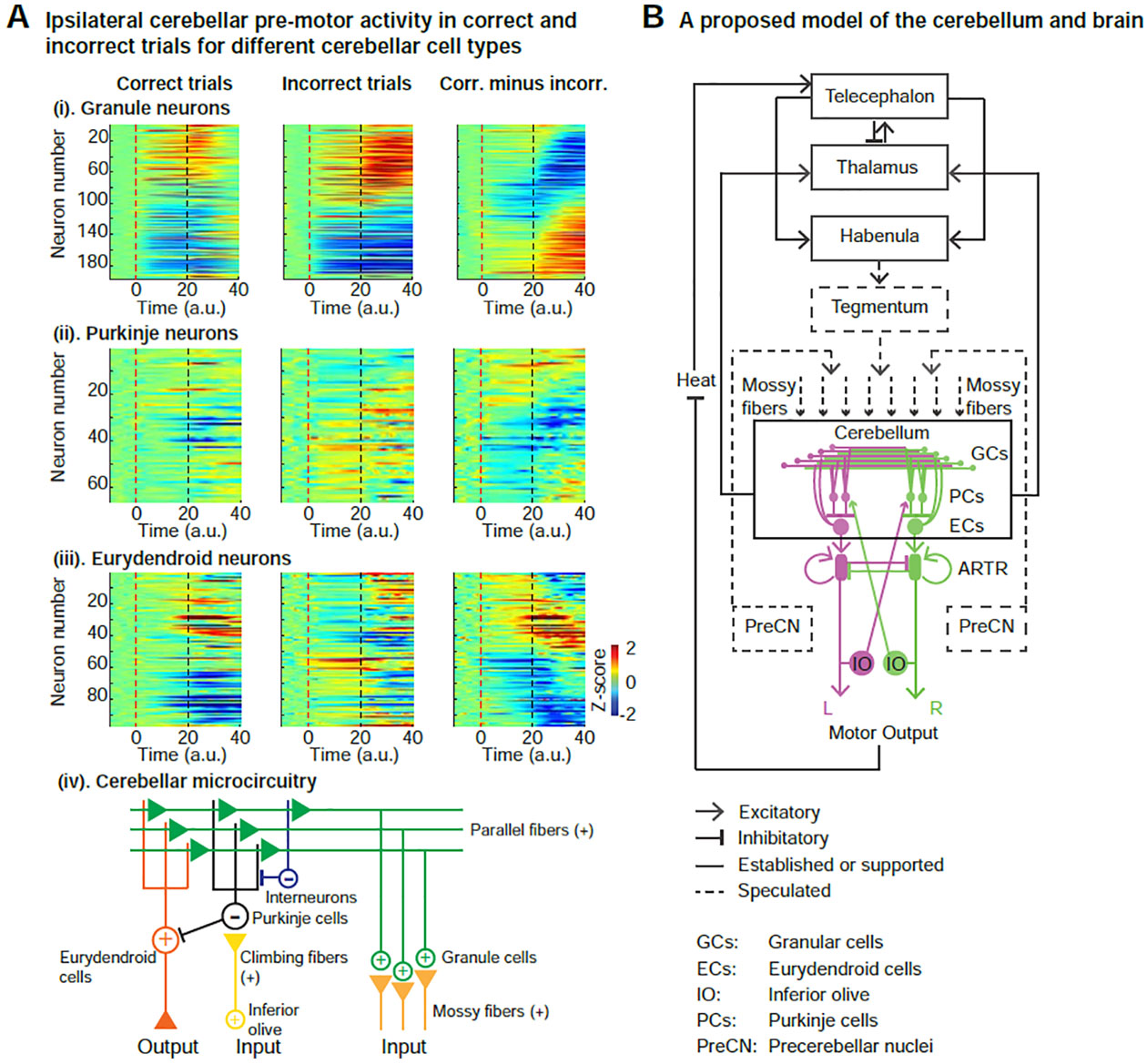
(A) Trial-averaged ipsilateral cerebellar activity for different cell types (granule, Purkinje and eurydendroid cells). Dashed line: red for heat onset; black for turn initiation. Only cells showing a significant difference in activity between correct and incorrect trials (p<0.001, t-test) are displayed, which accounted for >70% of the total recorded cells within each cell type. Left panels: correct trials. Middle panels: incorrect trials. Right panels: difference in average activity between correct and incorrect trials.

(i). The granule cells display the strongest observed pre-motor activity, as well as post-turn activity both in correct and incorrect trials.

(ii). The Purkinje cells display weaker pre-motor activity, especially in correct trials, compared to the granule cells. However, post-turn activity averaged across neurons is significantly higher in incorrect trials (p < 0.05, one-tailed Wilcoxon rank sum test).

(iii). The eurydendroid cells display some pre- and post-motor activity, driven by input from granule cells.

(iv). Diagram of the cerebellar microcircuitry. The main cerebellar inputs are the mossy fibers from various brain regions and the climbing fibers from the inferior olive. The activity of the granule cells (Figure 6A (i)) provides excitatory input via the parallel fibers to the Purkinje and eurydendroid cells, as well as inhibitory interneurons, which can suppress Purkinje cells and thus enable excitation of eurydendroid cells via the parallel fibers.

(B) Schematic overview of the proposed neurocircuitry underlying sensory information integration, learning, motor planning and action selection in our task: The heat stimulus activates the telencephalon, which inhibits thalamic activity and activates the habenula, which can regulate learning, reward prediction and the brain state. The cerebellum integrates this multimodal information, as well as that of various precerebellar nuclei, via the mossy fibers to prepare and generate movements. Cerebellar dynamics are relayed to the ARTR via the eurydendroid cells, initiating a motor command. Following movement initiation, the cerebellum receives feedback from the inferior olive and sends motor information back to the thalamus, thereby forming a closed loop for learning.

DISCUSSION

Supported by the conjecture that brain-wide processing of information is necessary for goal-directed behavior, we have used an operant learning task to investigate the neural basis underlying decision making in larval zebrafish. The combination of our behavioral assay with high-speed whole-brain calcium imaging based on LFM has allowed us to capture global and local brain state dynamics at cellular resolution, and their relationship to behavior at the trial-by-trial level. Our combination of brain-wide imaging and neuronal population analyses has uniquely enabled the study of dynamic changes in functional connectivity that occur on the timescale of seconds to minutes and are predictive of variability in decision timing and outcome, which could be masked by the requirement of averaging across task repetitions to reduce noise (Figure S6). Based on our observations and the known connectivity of the involved brain regions, we propose a model for how sensory information is transformed into decision and motor signals, and how learning and reward prediction is facilitated in this process (Figure 6B). The telencephalon (Portavella and Vargas, 2005), thalamus (Komura et al., 2001; Zhu et al., 2018) and habenula (Andalman et al., 2019; Hikosaka, 2010; Lee et al., 2010; Matsumoto and Hikosaka, 2007) are known to be involved in the regulation of learning, reward prediction and internal brain states, and can instruct the cerebellum on action selection. Upon heat onset the sensory signal is relayed to the telencephalon (Figure 2E) which suppresses neuroactivity in the thalamus and activates the habenula, which displays ramping-like activity during the pre-motor period. These signals, as well as other sensory and motor signals, are integrated by the cerebellum through the mossy fibers. Following movement initiation, the cerebellum sends motor information back to the thalamus, thereby forming a closed loop. Likely because our assay involves a learning and motor planning component, the overall functional circuitry spans the entire brain (Figure 6B), in contrast to a heat-evoked sensorimotor transformation which involves a hindbrain local circuit, yet also shows a strong response to heat in the telencephalon and the habenula (Haesemeyer et al., 2018).

This input to the cerebellum could be further amplified by the divergent mapping of the mossy fiber input to the granular cells (Huang et al., 2013; Ito, 2006; Li et al., 2013) and then integrated by the eurydendroid neurons (Ito, 2008) and fed into the ARTR, i.e. the hindbrain oscillator (Figure 6B). The underlying divergence of this circuitry at the level of the granular cells, their abundance in the cerebellum (Ito, 2006) and the observed pre-motor ramping activity explain our observation of the neuronal participation model (Figure 6B) and accounts for the granular cells as a main source of ramping. On the other hand, the observed contribution to the ramping by a small neuronal population with a gradual increase of activity (Figure S5D) can be explained by the activity of the ARTR neurons, which presumably receive input from the eurydendroid neurons. This notion is also directly supported by the observation that this small neuronal population is anatomically overlapping with the ARTR neurons (Figure S5E).

The bilateral relationship of the cerebellar neurodynamics that are predictive of turn direction and DT can be explained within a ‘competition-cooperation’ framework, in which turn directions are determined by the difference in neuroactivity between the ipsilateral and contralateral hemispheres, and the rate of bi-hemispheric population ramping activity predicts the DT. After motor response, two feedback signals are sent: The inferior olive activates the contralateral Purkinje cells via climbing fibers (Apps and Garwicz, 2005), while a self-excitatory ipsilateral feedback is sent to the ARTR (Dunn et al., 2016). The signal to the contralateral Purkinje cells can serve as an error signal that, together with inputs from other brain areas, facilitates synaptic plasticity (Albus, 1971; Apps and Garwicz, 2005; Dempsey and Sawtell, 2016; Marr, 1969). The preparatory activity, i.e. the neural signature underlying motor planning and decision making (Churchland et al., 2010; Svoboda and Li, 2018), is not an innate feature but emerges during learning of a task that requires optimization of expected reward for different possible actions (Wagner et al., 2019). We demonstrate this explicitly by showing that our observed cerebellar ramping activity uniquely emerges through our ROAST paradigm rather than representing an innate pre-motor activity feature of the cerebellum as it is absent in trials prior to training (Figure 3B (iv)). In mammals, the neuronal processes underlying decision making and preparation of goal-directed movements have been mainly attributed to the cortex (Miller, 2000; Shenoy et al., 2013; Svoboda and Li, 2018), while motor coordination functions, such as fine motor control and execution have been traditionally associated with the cerebellum (Glickstein, 1993; Manto et al., 2012). Our observations and interpretations are consistent with a number of recent studies which have challenged the traditional views of the cerebellum by providing evidence for cognitive functions such as in learning, language, evidence accumulation and reward prediction (Deverett et al., 2019; Giovannucci et al., 2017; Raymond and Medina, 2018; Schmahmann and Sherman, 1998; Sokolov et al., 2017; Strick et al., 2009; Timmann and Daum, 2007).

STAR METHODS

LEAD CONTACT AND MATERIALS AVAILABILITY

Further information and requests for resources should be directed to the lead contact, Alipasha Vaziri (vaziri@rockefeller.edu). This study did not generate new unique reagents.

EXPERIMENTAL MODEL AND SUBJECT DETAILS

Animal Subjects

Experiments were carried out in accordance with protocols approved by the Institutional Animal Care and Use Committee. Zebrafish (Danio rerio) lines used in this study for imaging and behavioral experiments were 7–9 day-post-fertilization Tg(elavl3:H2B-GCaMP6s) (Vladimirov et al., 2014) in Nacre or Casper mutant background. Adult fish were housed in a facility at 28.5 °C with lights on between 8 am and 10 pm. No statistical methods were used to pre-determine sample size.

METHOD DETAILS

Whole-brain Calcium Imaging with the Operant Conditioning Task, and Signal Extraction

7–9 day-post-fertilization zebrafish larvae were embedded in 2–2.5% low-melting-temperature agarose in a custom-made chamber on a glass slide and then immersed in fish water. The agarose around the tail, caudal to the swim bladder, was removed to free the tail of the larvae and then incubated for 6–8 hours for further solidification. Under this head-fixed condition, larvae were placed above a camera (Grasshopper3, PointGrey) for tracking tail movements at 160 Hz and placed under a 20×/0.5-NA water-immersion objective (Olympus) for whole-brain calcium imaging with an upright light-field microscope at 10 Hz (Nöbauer et al., 2017; Prevedel et al., 2014). The tail was illuminated with a near-infrared (NIR) 950 nm light-emitting diode (LED), and GCaMP was excited with a blue LED (pe-2, CoolLED). Custom-written MATLAB (MathWorks) software was used to extract the tail angle, using the resting tail position as the reference, with positive angles representing right turns and zero degrees corresponding to a straight tail. Heat stimulus was delivered using 980-nm fiber-coupled laser (Roithner Lasertechnik), collimated via a collimator (Thorlabs, F220FC-1064) and then projected to the head of the fish along the midline, with the spot diameter of 2.0 mm (measured power: 300 mW). A 950-nm bandpass filter (FB950–10, Thorlabs) was placed in front of the Grasshopper camera to reject scattered visible light and crosstalk from the heat stimulus. Real-time heat stimuli were controlled by a data acquisition board (USB-6008, National Instruments) and modulated by the extracted tail angle exceeding a threshold (35°) in a closed loop. For movement events with multiple tail deflections, only the first deflection was considered.

Image acquisition of the LFM was controlled using Micro-Manager (Stuurman et al., 2007) and triggered by the custom MATLAB software. The whole setup was controlled from a dual-CPU workstation (Z820, HP). 3D reconstruction of the LFM images was carried out offline with the volume of ~700 μm × 700 μm × 200 μm with 51 z-planes and fed into a custom-written pipeline for neuronal signal extraction based on the approach proposed by (Mukamel et al., 2009; Prevedel et al., 2014): The reconstructed LFM data, which is a timeseries of volumetric frames, was first de-trended by dividing each volumetric frame by a slowly-varying fit to the frame means. To reduce the data to an amount tractable by Independent Component Analysis (ICA), the variance over time was computed for each voxel, and the highest-variance voxels, as well as 2–3 continuous time ranges amounting to 10% of the total recording time were selected to serve as input data to the ICA. The entire recording volume was divided into 6 slightly overlapping sub-volumes. The selected voxels and timepoints were factorized independently for each sub-volume using the FastICA algorithm (initialized by PCA) (Hyvärinen and Oja, 2000), resulting in a set of spatial filters and associated temporal signals. The spatial filters were thresholded to detect regions of interest (ROIs), and ROIs compatible with shape and size of neurons were kept. Duplicate ROIs in the overlapping sub-volume regions were merged, resulting in the final set of neuron spatial filters. Finally, the corresponding neuron activity signals were extracted from the original reconstructed LFM dataset by summing (for each timestep) over the voxel brightness values in each neuron spatial filter.

Training Protocol and Animal Behavior

We aimed to find a robust behavioral paradigm that involved learning and short-term memory while exhibiting a delay period from the onset of an instructing sensory cue to the execution of motor response, during which the neuronal basis of motor planning and decision making could be studied. While previously used assays in larval zebrafish for sensorimotor transformation lack the above features, most of the typically used assays in rodents or primates study motor planning by introducing a delay period from the onset of the stimulus to a go cue, after which the animal is trained to initiate a motor response (Mohebi and Oweiss, 2014; Shenoy et al., 2013; Svoboda and Li, 2018). However, motor responses of animals engaged in naturalistic action selections are self-initiated and happen in the absence of a go cue. The ROAST operant conditioning paradigm (Figure 1A) addresses both issues. Typically, each recording consisted of 20–25 trials and lasted for one hour. In each trial, heat stimulus was delivered 5 seconds after the trial started and was terminated immediately when a turn in the correct direction exceeded a threshold (35 degree). If an animal failed to make a correct movement within 100 s, the laser was switched off and the fish received a 20 s break before the start of the next trial. Otherwise, if an animal made a correct movement, the heat stimulus was turned off and the fish received a break for the rest of the 100 s trial. The full training protocol for each fish consisted of two training blocks (one left- and one right-training block), with each block containing 20–25 trials. Since individual fish exhibited a bias for a specific direction (Li, 2013), the reward direction in the first training block was chosen against this bias and was subsequently reversed in the second block. Prior to the first block, 3–5 probe trials were conducted to determine the pre-existing bias of individual fish. For “learners” (see below), the same larvae were imaged twice for two training blocks, over a total of two hours, and with a 0.5 h break in between. A given trial was classified as correct when the first heat-evoked turn of the animal was in the reward direction, and a fish was defined as a “learner” when the asymptote of the learning curve (modelled by a sigmoidal function that was fit to the outcomes) in both blocks reached a threshold of 70% correct. Fish that learned in the first but not in the second block were defined as intermediate learners and their data was not included in the data analysis. If a fish failed to learn in the first block, it was categorized as a non-learner and was not considered further for the second training block. Overall, we behaviorally trained and recorded data from 26 larvae resulting in 39% learners, 46% non-learners and 15% intermediate learners, which were not included in further analyses. In all further analyses, training blocks were analyzed separately, such that a “correct trial” always corresponded to a turn in the left or right direction.

Pre-processing of the Neuronal Signals

Each neuronal time series was de-trended individually to correct for photo-bleaching, and then normalized as ΔF/F0 = (F-F0)/F0, where F is the fluorescence of the neuron at a given timepoint and F0 is the average fluorescence of the neuron across the entire recording. Noise was removed via total variation regularization by calculating the cumulative sum of the de-noised time derivatives (Chartrand, 2011). The de-noised time series X of each neuron were then normalized by taking the Z-score, given as (X – mean(X))/SD(X), for further analysis. This pre-processing procedure and subsequent analyses were performed using MATLAB (MathWorks).

Behavior Classification

In addition to online tracking, offline behavioral classification was used to classify the tail movements as left turns, right turns, and struggles (or swimming), using a method similar to the one described by (Haesemeyer et al., 2018). Briefly, since larval zebrafish move in bouts rather than swim continuously, and since the bout duration lasts for about 250–400 ms in head-restrained fish (Severi et al., 2014), the movement bout was detected by scanning through the time series of the tracked tail angle in a sliding window of 50 frames (corresponding to ~312 ms at a frame rate of 160 Hz). Within the time window of one bout, the time of movement initiation was set to the timepoint when the tail angle exceeded 5° for the first time. Then, the bias of tail movements was calculated, and the bout was categorized as a unilateral ‘turn’ or a bilateral ‘struggle’ with the threshold of bias at 1.05. The turn direction was determined from the sign of the tail angle, negative or positive, for left and right turns (labelled “TurnL” and “TurnR”), respectively.

Decision Time

Decision time (DT) was measured as the time between heat onset to the initiation of the first turn, regardless of correct or incorrect outcome, in a given trial. Because the temperature changes from the heat stimulus became relatively stable 5 s after heat onset, only trials with DT longer than 5 s were used, to minimize stimulus-related variation across trials.

Performance-dependent Bifurcation of Brain States

To visualize the temporal evolution of brain states towards correct versus incorrect decisions, the time-dependent correlation (Pearson’s r) was calculated between each brain state in a trial and a reference brain state determined by averaging all brain states of the same type (i.e., correct versus incorrect). Partial correlation coefficients were utilized to factor out the heat-induced neuronal contribution both in correct and incorrect trials.

Partial Correlation Coefficients

The partial correlation coefficient r of X and Y while controlling for the effect of Z is given as:

$$r_{XY\cdot Z}=\frac{r_{XY}-r_{XZ}{r}_{YZ}}{\sqrt{\left(1-r_{XZ}{}^2\right)\left(1-r_{YZ}{}^2\right)}}$$

Here, r_XY is the pair-wise correlation coefficient:

$$r_{XY}=\frac{\mathit{\text{cov}}\left(X,Y\right)}{{\sigma }_X{\sigma }_Y}$$

Partial correlation coefficients were computed in MATLAB (MathWorks), using the function partialcorr().

t-SNE on the Brain States

t-Distributed Stochastic Neighbor Embedding (t-SNE) (Maaten and Hinton, 2008) was applied to the sequence of brain states, where each “brain state” input vector was the activity state of all neurons at a given timepoint. Briefly, t-SNE transforms the structure contained in high-dimensional data into a two- or three-dimensional map by minimizing the Kullback-Leiber divergence between the Gaussian similarity matrix of the data points and the t-distributed similarity matrix of the map points. t-SNE maintains the local structure by keeping similar data points close to each other on the t-SNE map (Maaten and Hinton, 2008). Even though t-SNE has the disadvantage of not providing the same visualization on each run of the optimizer, nor an explicit transformation matrix that would be required to establish a quantitative correspondence between the t-SNE map and neuroanatomy, it nevertheless provides an effective, exploratory tool for identifying hidden, low-dimensional structure in high-dimensional data (Davie et al., 2018; Grün and van Oudenaarden, 2015; LeCun et al., 2015; Macosko et al., 2015). Brain states consisting of 25,000 to 35,000 input vectors were mapped onto a 2D t-SNE map using value of 1000 for the “perplexity”, which is a critical hyper-parameter in t-SNE. Other values for perplexity, such as 500–2000, gave similar results. t-SNE maps from different animals were normalized to [0,1] in both the x- and y- dimension. Pair-wise distances of all pairs of brain states were measured by their Euclidian distance in the 2D t-SNE map.

t-SNE on the Neuronal Space

To highlight task-relevant activity, we embedded regressors of the behavior and the heat stimulus into the neuronal space as “baits”. We defined four regressors: “Turn L”, “Turn R”, “Heat ON” and “Heat OFF”, obtained by convolving the actual time series of each regressor with the temporal response kernel of our calcium sensor (NL-GCaMP6s). Then t-SNE was applied to the “neuronal space”, where each input vector was the normalized time series of one neuron in one recording, plus the four behavior- and stimulus regressors. 4000 to 6000 inputs were transformed into a 2D t-SNE map. Perplexity values ranging from 40 to 120 were tested and then chosen such that in the resulting map the regressors were mostly well-separated. Hierarchical clustering was then performed on the chosen t-SNE map using the criterion of Ward’s minimum variance method (Ward, 2012). The final number of clusters was determined as the smallest number of clusters such that the top three principal components of each cluster explained more than 80% of the variance, or the first component more than 50%, using principal component analysis (PCA).

Measuring Coordination and Integration Across Brain Regions

Correlation was used as a quantitative metric of coordination and integration (Cohen and Kohn, 2011; Kohn et al., 2016). Brain regions were defined using the functional clusters identified using t-SNE on the neuronal space (see above). Specifically, the absolute value of the mean pre-motor correlation between all pairs of neurons across two brain regions was calculated for each trial. The period over which the correlations were calculated lasted from 10 seconds before heat onset to 1 second before movement initiation. Significant differences between correct and incorrect trials in all pairs of brain regions were measured using a two-tailed t-test. For each pair of brain regions, the average difference in absolute correlation was calculated by comparing the average across all correct trials to all incorrect trials. Similar quantities were measured by splitting trials into pre- versus post-learning, as identified by the inflection point of the sigmoid function representing the learning curve (described above), instead of correct versus incorrect trials.

Identification of the Neurons of Cerebellum and ARTR for Further Analysis

Due to individual differences in neuroactivity and learning performance, the neurons in the cerebellum and ARTR did not always end up in the same locations in the t-SNE neuronal spaces across animals. To ensure that the analysis was always performed on the medial portion of cerebellum and ARTR across animals (Figure 4–5), the neurons in these regions were selected manually based on anatomical landmarks (Dunn et al., 2016; Randlett et al., 2015; Takeuchi et al., 2015).

Population Dynamics using Demixed PCA (dPCA)

dPCA was performed on neuronal populations, following instructions described previously (Kobak et al., 2016). Briefly, dPCA decomposes the activity of a neuronal population into a few task-related components, such as different stimuli and decisions. Thereby, besides identifying the transformation and components that account for the majority of the observed variance in the data as in PCA, dPCA can also reveal the dependence of the neuroactivity on task-related parameters such as stimuli states and decisions. The goal of dPCA here was to project population dynamics into a small number of dimensions that capture more than 80% of the variance and to decode decision-dependent versus decision-independent components.

Briefly, for each neuron in a given recording, the time series was divided into correct and incorrect trials based on whether the first turn was in the correct direction. To be able to average trials of different decision times (DTs) in dPCA, time series from different trials were first aligned relative to two timepoints, 5 s after heat onset and after movement initiation, respectively, using a time warping process, with DT defined as 20 (a.u.) after alignment (Figure S3A). Note that only trials with DT ≥ 5 s were used for dPCA. The time window of each trial started 10 s before heat onset and ended 20 s after the first turn initiation. For each neuron in each trial, the average activity during the first 10 s was used as the baseline and subtracted from the time series. Because the movements were the only differing conditions across trials, two types of components were defined: decision-dependent components, from which the correct vs. incorrect trials could be decoded, and decision-independent components, in which the population dynamics in correct and incorrect trials followed the same patterns.

To examine whether individual decision-dependent dPCs could decode correct versus incorrect trials with statistical significance, we used each dPC as a linear decoder to assess their classification performance (Kobak et al., 2016). Cross-validation (n = 100) was used to measure time-dependent classification accuracy of the dPCs. Then a shuffling test (n = 100), which shuffled the identity of correct vs. incorrect trials without changing the neuronal time series, was used to assess whether the classification accuracy was significantly above 99% of the shuffled runs in 10 consecutive timepoints. Timepoints of significant decoding were marked with thick horizontal black lines in Figure 3A, 4A, S4B, S4C. The dPCs which were able to decode correct vs. incorrect trials before movement initiation were defined as pre-motor decision-dependent components.

Analysis of Pre-Motor Decision-Dependent Activity

To compare the ability for predicting decision directions between learners and non-learners, warped time series with a DT of 20 s were used and the same procedure as above was performed.

To measure the real timepoint of successfully predicted decision direction in learners, first warped time series were used to obtain the decoder of dPCA and the classification outcome from single-trials via cross-validation. Classification outcomes of single trials then went through an unwarping process by re-stretching back to the original DTs (Figure S3C). Classification accuracy from unwarped single-trial classification outcomes was obtained by aligning to the movement initiation time (Figure S3D(i–ii)). Error margins of classification accuracy were obtained from a shuffling test (n = 100) using the same procedure and were aligned to the movement initiation time after shuffling (Figure S3D(iii)). Time for predicting decision directions was defined as the earliest timepoint before movement initiation when the classification accuracy was significantly above 99% of shuffled runs in 10 consecutive timepoints (Figure S3D(iii)).

Analysis of Ramping Activity

The first dPC of the cerebellum and ARTR showed a temporal ramping activity during the period from heat onset to movement initiation across animals. To measure the velocity of the ramping activity, i.e. the ramping rate, dPCA was first applied to neurons in the cerebellum and ARTR from both hemispheres to obtain the decoder and encoder, and then the decoder from dPCA (Figure S3B) was used to transform the neuroactivity (without time warping) into the low-dimensional map space. Then, a linear fit was applied onto the first dPC from heat onset to 1 s before movement initiation in each trial, thus obtaining the ramping rate at the single-trial level (Figure S5A). Single-trial decision time (DT) was predicted at each timepoint t by obtaining the ramping rate (x) of dPC1 via a linear fit from 0 to t s after heat onset and utilizing a log-linear model log10(DT) = −3.94x + 1.66 (Figure S5B). Subsequently the predicted turn initiation timepoint is calculated by using DT – t (Figure S5B).

In order to demonstrate the decrease in prediction accuracy resulting from averaging data across multiple trials, we randomly sampled N = 19 trials with replacement from an example fish and calculated the average ramping rate and average decision time (Figure S6A). An identical log-linear model as above was fit to the trial-averaged ramping rates and decision times, which was then utilized to predict the decision time in single trials (Figure S6B).

To investigate the degree to which an increasing pool of active neurons was the driver of the observed ramping activity, we first classified the states of activity of each neuron at a given timepoint in a binary fashion as “active” or “inactive” depending on whether its activity was above or below its own standard deviation (SD). We then determined the degree of neuronal participation by calculating the fraction of active neurons at each timepoint and compared this to the population activity, as reported by dPC1, as a function of time. We compared this to the scenario in which the ramping activity would be explained by an increasing level of activity of individual neurons. To do so, we used linear correlation to measure the similarity of activity of all individual neurons to the population ramping during the pre-motor period, obtained the correlation coefficients for each neuron, calculated the distribution of these correlations and compared this distribution to the correlation obtained between the neuronal participation and the population ramping.

Analysis of Ipsi-Contra Interaction

To examine whether there existed interaction and competition between hemispheres, dPCA was applied to neurons in the cerebellum and ARTR from both hemispheres to obtain the decoder and encoder, and then this decoder from dPCA was used to transform the neuroactivity (without time warping) into the low dimensional space. Since the response of each neuron can in principle be tuned to both features of the stimulus and of the motor output, a bilateral differential activity between the hemispheres during the pre-motor period may be masked by other stronger signals in the cerebellum and ARTR, such as the decision-independent dPC1. Thus, to increase the sensitivity of the analysis, neuroactivity containing only the pre-motor decision-dependent component was used. To do so, only the pre-motor decision-dependent component with the corresponding encoder was used to reconstruct the neuroactivity (Figure S4D). With these two linear transformations, neuroactivity was obtained that was predictive for movement direction with temporal and spatial information. Then the neurons were pooled according to ipsilateral or contralateral location based on their anatomical locations in the fish brain, and their activity was averaged across pools. A time window from −4 to −2 s (note that this was the unwarped time) before turn initiation was used, which was within the time window of 5 s decision time as the threshold. The separation of 2 s from turn initiation was chosen to avoid any influence of post-turn activity from the de-noising process since de-noising by total variation regularization leads to a smoothing of the time series. The averaged activity of the ipsilateral and contralateral cerebellum and ARTR were then compared at the single-trial level.

Two-Photon Imaging in Specific Cerebellar Cell Types

Two-photon imaging experiments were performed on a Scientifica Slicescope platform with a 20x/1.0-NA water-immersion objective (Olympus). The two-photon excitation source (Coherent Chameleon) delivered 140-fs pulses at an 80-MHz repetition rate and 960-nm wavelength (measured power: 5–12 mW). The beam intensity was controlled via an electro-optical modulator (Conoptics) for attenuation and blanking, and fed into a galvo-based scan head (Scientifica). Fluorescence from the sample was detected by a non-descanned photomultiplier tube (PMT), which consisted of an infrared blocking filter, collection lens, 565LP dichroic, 525/50-nm and 620/60-nm emission filters, and Scientifica GaAsP (green channel) and alkali (red) PMT modules. Experiments were controlled with Scanimage (Vidrio Technologies). Typical cerebellar recordings imaged ~430 × ~215 × 80 μm with 6–8 z-planes at a volume rate ~0.8 Hz. Neuron ROIs and activity were detected using CaImAn-MATLAB (Giovannuci et al., 2019).

Granule cells of the cerebellum were imaged using Tg(gSA2AzGFF152B; UAS:GCaMP6s) (Filosa et al., 2016; Knogler et al., 2017; Takeuchi et al., 2015). Purkinje and eurydendroid cells were imaged using Tg(Huc:H2B-GCaMP6s; GAD1b:RFP) (Freeman et al., 2014; Satou et al., 2013). Purkinje cells were isolated by manually selecting identified neurons expressing Gad1b:RFP in FIJI, and the remainder of the GCaMP-expressing cells in the dorsal cerebellum represented the eurydendroid cell population. Decision-dependent cells were identified by performing a t-test between their distribution of single-trial pre-motor activity in correct versus incorrect trials. Single neuron average activity traces were calculated for representative fish by aligning the activity to heat onset and movement initiation and then averaging over correct or incorrect trials. The difference in average activity between correct and incorrect trials was calculated as a function of time for each neuron in order to highlight any pre- and post-motor decision-dependent changes.

Two-Photon Lesions in Targeted Brain Regions

Two-photon lesions of the telencephalon and habenula were performed using our Scientifica two-photon platform on fish that had learned (see criterion below) in the first training block. An area of ~25 × 25 μm was lesioned with a power of ~60 mW for ~1.2 seconds. If necessary, lesions in the same area were repeated until a hole in the tissue was observed. An identical procedure was performed on both hemispheres. After lesioning, the second training block was performed with the reversed reward direction. In the control group, fish that had learned (see criterion below) in the first training block were trained in the second training block, without lesion.

Lesions of the cerebellum were performed on fish that had learned (see criterion below) in the two training blocks. The same protocol for lesion was performed. Ipsilateral lesion referred to a lesion in the training side, while contralateral lesion referred to a lesion in the opposite side of the training direction, and bilateral lesion was the same procedure for both hemispheres.

Analysis of Spontaneous Freely Behaving Swimming Behaviors

Analysis of spontaneous turn preference before and after unilateral cerebellum lesions was performed by recording turn direction in freely behaving zebrafish in 3.5cm circular chambers for 1 hour. Behavioral tracking was performed using DeepLabCut 2.0 (Nath et al., 2019) and the number of left and right turns, identified by measuring a leftward or rightward change in orientation between the start and end of each swim bout, were counted for each fish.

QUANTIFICATION AND STATISTICAL ANALYSIS

A total of 26 larvae were trained under the ROAST assay and 5 larvae went through spontaneous movement with LFM imaging. LFM data from two-block learners, non-learners and fish exhibiting spontaneous movements – but not the data from intermediate learners – went through the 3D reconstruction. Subsequently, our signal extraction pipeline was applied to the reconstructed LFM images. We found imaging results and data quality to be reliably reproducible and consistent, both across imaging sessions with the same animal, and across animals. All statistical tests and sample sizes in the imaging and lesion studies are described in the corresponding figure captions.

DATA AND SOFTWARE AVAILABILITY

Our custom data-processing pipeline for LFM data is available for download. Software for data analysis, as well as data, is available from the corresponding author upon reasonable request.

Supplementary Material

1

Figure S1. An operant conditioning assay for larval zebrafish combined with whole brain calcium imaging. Related to Figure 1.

(A) Latency to relief from heat decreases as a function of trials. Data averaged from both blocks of 10 learners (mean ± SEM). Dots indicate single trials. Two tailed *p = 0.048, Kruskal-Wallis test. Black dots indicate individual trials.

(B) Decision time (DT), defined as the time from heat onset to movement initiation, as a function of trial number remains constant. Data averaged from both blocks of 10 learners (mean ± SEM). Dots indicate single trials. Two-tailed p = 0.99, Kruskal-Wallis test.

(C) Dynamic evolution of brain states, i.e. the activity of all neurons at a given timepoint, at different task epochs.

(i) During the initial 15 s of Heat ON, the forebrain neurons show increased activity; white arrow heads: habenula (Hb); red arrow heads: telencephalon (Te).

(ii) For Heat ON > 15 s, the activity in the ipsilateral cerebellum (Cb, white arrow) increases, while the thalamus (Th, yellow arrow heads) decreases.

(iii) At correct turn initiation, the ipsilateral cerebellum and ARTR are highly active (white arrow and arrowhead, respectively).

(iv) During initial 15 s of Heat OFF, the activity of the ipsilateral cerebellum (white arrow), but not ARTR (white arrowhead), decreases, while that of the contralateral cerebellum, ARTR, telencephalon and the thalamus (yellow arrowheads) increases.

(v) All neuroactivity reaches the baseline levels again for longer periods after Heat OFF. Color-coding shows averaged brain states during same epochs across trials; spatial filters of neurons are maximum-projected and superimposed on average fluorescence for anatomical reference. Same dataset as Figure 1D. Scale bar, 50 μm.

(D) The numbers of exacted neurons from different brain regions are consistent across animals and recordings. n = 10 recordings from 5 animals. In each recording, the number of exacted neurons is 5265 ± 224 in total, 1631 ± 121 from the forebrain, 1450 ± 152 from midbrain, and 2183 ± 78 from hindbrain, mean ± SEM.

(E) The number of extracted neurons across the axial range is consistent across animals and recordings. One example dataset and n = 10 recordings from 5 animals display similar distribution along the axial range, which corresponds to the dorsoventral axis of the zebrafish.

(F) Ineffective separation of neural dynamics at different task epochs by principal component analysis (PCA). Brain states represented as the top three principal components (PCs) as a function of time. Same data as Figure 1D and 2C. Viewing angle is chosen in attempt to distinguish post-correct versus post-incorrect turn activity, which is not possible. This is consistent with the observation that the first three PCs captured <60% of the variance of the brain dynamics (Figure S1G). As the brain states are high-dimensional, only visualizing the top-ranking PCs is not informative, unless lower-ranking PCs are further examined in separate plots. An alternative method for dimensionality reduction and visualization is required.

(G) Cumulative explained variance of brain states as a function of number of PCs included. The brain states are high-dimensional, since explaining 80% of the total variance requires 15 dimensions.

2

Figure S2. Decision making relies on coordination and integration of distributed information across the whole brain. Related to Figure 2.

(A) Dynamic evolution of brain states visualized in a 2D t-SNE map, with major transitions in brain states associated with Heat ON (red and yellow points) and Heat OFF (black and blue points). Brain states (n = 24,472) from 25 repeated trials in an example fish represented as dots, color-coded by the stimuli. The heat stimulus drove temporally sharp transitions between the ON and OFF states, as well as continuous evolution during each individual state, and the sequences of these global states were to a certain degree stereotypical before and after motor behavior.

(B) Similarity of brain states within and across Heat ON and OFF. Within-epoch brain states show a higher level of similarity than across-epoch, calculated as the pairwise Euclidean distances between brain states in t-SNE space. Left: an example learner. Right: same for multiple animals (n = 12). ***p < 0.001, Wilcoxon rank sum test.

(C) Brain states at movement initiation exhibit a higher level of similarity than brain states on average with the “Heat ON” cluster, as measured with the Euclidean distance between brain states in t-SNE space. Left: an example learner. Right: same for multiple animals (n = 12). ***p < 0.001, Wilcoxon rank sum test.

(D) Brain states resulting in correct turns exhibit a higher level of similarity at movement initiation than those resulting in incorrect turns, as measured with the Euclidean distance between brain states in t-SNE space. Thus, correct behavior is associated with lower variability in brain state space. Left: an example learner. Right: same for multiple animals (n = 12). Wilcoxon rank sum test.

(E) Example behavior and stimulus regressors obtained by convolving behavior and stimulus time traces with the nucleus-localized (NL)-GCaMP6s kernel. These regressors were processed by t-SNE together with neuroactivity traces. This approach allowed to establish a link between functional neuronal clusters, task relevant states (behavioral and stimulus) and brain anatomy by mapping of the clusters to different brain regions (Figure 2E).

(F) Brain-wide pre-motor activity correlations suggest the coordination and integration of information during correct trials. Left: Difference in average absolute correlation between correct (Corr.) and incorrect (incorr.) trials, among functional clusters. Right: Difference between post-learning and pre-learning trials. The ipsilateral cerebellum displays significant increase in the correlation with itself and the habenula during correct trials compared to incorrect trials, which is absent when comparing pre-learning versus post-learning trials. The telencephalon shows significant changes in correlation with the contralateral cerebellum when comparing correct versus incorrect trials, and with the ipsilateral cerebellum when comparing pre-learning versus post-learning trials. Two-tailed t-test, *p < 0.05, **p<0.01.

3

Figure S3. Applying demixed PCA (dPCA) on the population neuroactivity to decode and predict decision directions. Related to Figure 3.

(A) Time warping procedure to align trials with different decision times for dPCA. To prepare the neuronal time series from different trials for dPCA, we define two alignment timepoints – T1, 5 seconds after heat onset, and T2 at turn initiation. These timepoints are chosen such because the temperature becomes relatively stable 5 seconds after heat onset and in order to strictly avoid any contaminations from signals during post-turn period. For each trial, we find these two timepoints T1 and T2, and stretch or compress the neuroactivity between T1 and T2 to 15 arbitrary units (a.u.), thus making the decision time 20 a.u., which is chosen based on the average decision time of ~20 seconds. After this warping procedure, neural time series from different trials can be analyzed by dPCA to obtain the decoder and encoder. Furthermore, as the decision time for each trial is known, this process is reversible, and demixed principal components (dPCs) can be stretched back to the original, i.e., unwarped time. For prediction of time, decision time-related and ramping-related analyses (such as Figure 3D, 4 and 5), we use real timestamps instead of the warped ones.

(B) Flowchart for decomposing neuronal population activity into task-related components, i.e. decision-dependent and decision-independent, by dPCA. This flowchart illustrates the process of compressing and decompressing the population activity through two linear transformations. The compressing step via the decoder provides the latent dPCs, the decomposed low-dimensional population dynamics. The decompressing step via the encoder transforms dPCs back to the space of neuronal time series.

(C) Schematics of single-trial prediction for decision direction based on real time by an unwarping procedure.

(i). Classification of decision direction as a function of time using warped time with a linear classifier on the decision-dependent dPCs. Green and magenta curves: trial-averaged dPCs from trials as the training data, correct and incorrect trials, respectively. Black curve: single-trial dPC from the test trial. Classification is done by comparing the distance between the test trial and correct versus incorrect trials at each timepoint.

(ii). Classification outcome, true or false, at each timepoint of the test trial, in warped time. (iii) Real time prediction outcome, using a second time warping process which is reversed to panel (A).

(D) Predicting decision directions for learner fish.

(i) Examples of binary prediction at the single-trial level.

(ii) Mean prediction accuracy as a function of time, obtained by aligning the binary prediction from all the trials to the movement initiation. Due to different decision times, the timepoints of heat onset are not aligned. Data from an example learner.

(iii) Prediction timepoint is defined as the earliest timepoint (red dot) when classification accuracy (light blue curve) exceeds 99% of the shuffling tests (light shaded area) in 10 consecutive timepoints. n = 100 shuffling tests; dark blue line and shaded band: mean and SD of shuffling tests.

4

Figure S4. Ipsilateral-contralateral competition in the cerebellum determines the decision outcome. Related to Figure 4.

(A) Averaged task-related dPCs from multiple fish (mean ± 1.96SEM, n = 9). The patterns of the dPCs across multiple fish are consistent with the example in Figure 4A.

(B) Task-related dPCs from non-learner fish. Decision-independent dPC1 (heat-evoked ramping signal) and dPC3 (heat-and-motor-evoked signal) are similar to the example learner (Figure 4A); decision-dependent dPCs, the post-turn feedback signal as represented by dPC2, is similar to that of the learners (Figure 4A); dPC4, the pre-motor component, appears weaker than the learner (Figure 4A), and not predictive of the future turn direction. dPCs are displayed as mean ± 1.96SEM across trials.

(C) Task-related dPCs from fish performing spontaneous movements. No stimulus is delivered in this task. Decision-independent dPC1 and dPC3 are almost absent, without pre-motor ramping or plateau, while a weak post-motor separation by the dPC2 is present. Pre-motor dPCs in spontaneous turns are not predictive of turn direction. Decision-dependent dPC4 is absent.

(D) Illustration of the workflow for reconstructing neuroactivity from pre-motor decision-dependent dPCs only. dPC4 is used for reconstruction based on the results shown in Figure 4C–E.

(E) Comparison of reconstructed neuroactivity during pre-motor periods between ipsilateral and contralateral cerebellum on a trial-by-trial basis, from an example non-learner. Pre-motor activity is averaged from 4 to 2 s before turn initiation in order to avoid any contamination from post-motor activity. Unlike the example learner, the neuroactivity on the ipsilateral side of the non-learner is not significantly different from the contralateral side in both correct and incorrect trials. Wilcoxon signed rank test, two-tailed.

(F) Comparison of the ipsilateral-contralateral activity at the single-trial level from trials pooled across multiple non-learners. The ipsilateral pre-motor activity is not significantly different from the contralateral side during correct trials. Wilcoxon signed rank test, two-tailed.

5

Figure S5. The ramping rate of bilateral cerebellar population dynamics determines decision. Related to Figure 5.

(A) An example of how ramping rate of a given trial was evaluated. A linear fit is applied to the ramping activity from heat onset to 1 s before turn, using real time. The slope parameter is used as the ramping rate.

(B) Illustration of the prediction of movement initiation time at a given time after heat onset in a given trial. The movement initiation time is predicted from the ramping rate, determined as in panel (A), using a log-linear model fit to the data shown in Figure 5C.

(C) Three example neurons to illustrate the complex forms of pre-motor and post-motor activity across trials, and more importantly pre-motor ramping is not present in these neurons at the single-trial level. Warped time series (See Figure S3A) are used to show and compare multiple trials.

(D) Distribution of correlation between activity from single neurons and population ramping activity. 82% of the neurons show correlation < 0.799, hence only 18% of neurons exceed the correlation between neuronal participation ratio and population activity. In other words, ramping activity is better explained by the level of neuronal participation than by individual neurons.

(E) Anatomical location of the neurons (top 18% in (D)) whose correlation coefficients to population ramping activity exceed the correlation between degree of neuronal participation and population activity. These neurons mainly overlap with the ipsilateral ARTR, colored red. Other active neurons from the rest of the cerebellum and ARTR are indicated in yellow. Scale bar: 50 μm.

6

Figure S6. Trial-averaged methods are unable to accurately predict decision time. Related to Figure 5.

(A) Averaging across trials removes the strong correlation between ramping rate and decision time, as was seen in Figure 5C. Average ramping rates and decision times are computed by randomly sampling trials with replacement from one representative fish (see STAR Methods). The inverse correlation between average ramping rate and average decision time is not significant, unlike in single-trial analyses (Figure 5B), with p > 0.05.

(B) A log-linear model fit to trial-averaged ramping rate and decision time is not able to quantitatively predict decision time from ramping rate. The model is built using a log-linear fit (as in Figure S5B) to trial-averaged data (shown in panel (A)), but predictions are made on the single-trial level as in Figure 5D. The lack of any significant correlation between average ramping rate and average decision time in panel (A) leads to systematic errors in the prediction of single-trial decision time. Data represent mean ± 1.96 SEM from 20 trials.

7

Movie S1. Projected volumetric reconstruction of whole-brain LFM calcium imaging data. Related to Figure 1.

Maximum intensity projections along three orthogonal directions of reconstructed LFM recording of GECI activity in an example zebrafish with pan-neuronal expression of GCaMP6s. Scale bar, 50 μm. Recording frame rate: 10 fps. Playback: 30× real time.

8

Movie S2. Single-trial bifurcation process during the pre-motor period. Related to Figure 2C.

Animation of the evolution of individual correct and incorrect trials during the pre-motor period (i.e., from heat onset to movement initiations), expressed as correlation with the averaged, final brain states at movement initiation. Black diamonds indicate heat onset, green and magenta dots indicate movement initiations for correct and incorrect turns, respectively. Color scale encodes temporal progress from heat onset to movement initiation. Note that these individual trials are with different decision times. Playback at 3× real time.

9

Movie S3. Predicting turn direction and turn time from neuroactivity at the single-trial level. Related to Figure 4–5.

Movie of calcium imaging data during a ROAST trial, together with evolution of prediction for both, turn direction and turn time. Prediction is obtained from the neuroactivity at the single trial level. The example is a correct trial, with the training towards the right direction. Video starts 5 s before heat onset and ends 5 s after movement initiation. The prediction is evaluated starting at heat onset and updated until movement initiation.

Top panels: Maximum intensity projections of neuron centroids, superimposed on an anatomical reference, Tg(elavl3:H2B-RFP) from the Z-Brain Atlas (Randlett et al., 2015). Filled red square indicates Heat ON, hollow red square indicates Heat OFF. Scale bar, 50 μm.

Middle panel: Outcome of a binary prediction for turn direction. Hollow triangles indicate the possible outcomes (left versus right), and filled triangles indicate predicted outcome, color coded green for the right (correct) side and magenta for the left (incorrect) side.

Bottom left panel: Evolution of error in predicted turn time, i.e. the difference between the prediction and the actual turn time. Red dashed line indicates heat onset; white dashed line indicates turn initiation. Bottom right panel: Plot of tracked tail segments (n = 9 segments). Each rendered frame is the maximum-projection of 16 consecutive recorded frames, to match behavioral recording frame rate (160 fps) to brain imaging frame rate (10 Hz). Playback is in real time (10 fps).

KEY RESOURCES TABLE

REAGENT or RESOURCE	SOURCE	IDENTIFIER
Experimental Models: Organisms/Strains
Tg(elavl3:H2B-GCaMP6s)	(Vladimirov et al., 2014)	N/A
Tg(gSA2AzGFF152B)	(Takeuchi et al., 2015)	N/A
Tg(Huc:H2B-GCaMP6s; GAD1b:RFP)	(Freeman et al., 2014; Satou et al, 2013)	N/A
Tg(UAS:GCaMP6s)	(Filosa et al, 2016)	N/A
Software and Algorithms
μManager	Open Imaging	https://micro-manager.org/
MATLAB (Behavioral and imaging analysis, modeling)	MathWorks	https://www.mathworks.com/products/matlab.html
FIJI (ImageJ) (Image Processing)	NIH	http://fiji.sc
Custom data-processing pipeline for LFM data	(Prevedel et al, 2014)	https://static-content.springer.com/esm/art%3A10.1038%2Fnmeth.2964/MediaObjects/41592_2014_BFnmeth2964_MOESM189_ESM.zip
Demixed Principal Component Analysis (dPCA)	(Kobak et al, 2016)	https://github.com/machenslab/dPCA
t-Distributed Stochastic Neighbor Embedding (t-SNE)	(Maaten and Hinton, 2008)	https://lvdmaaten.github.io/tsne/
Independent Component Analysis (FastICA)	(Hyvarinen and Oja, 2000)	https://research.ics.aalto.fi/ica/fastica/
Scanlmage	(Pologruto et al, 2003)	http://scanimage.vidriotechnologies.com/display/SIH/ScanImage+Home
CalmAn-MATLAB	(Giovannucci et al, 2019)	https://github.com/flatironinstitute/CaImAn-MATLAB
DeepLabCut 2.0	(Nath et al, 2019)	https://github.com/AlexEMG/DeepLabCut

Highlights:

• Whole-brain Ca²⁺imaging and decision making in larval zebrafish on the single-trial level

• Pre-motor bifurcation and trial-by-trial changes of functional connectivity

• Cerebellar activity predicts decision outcome and decision time >10 s before movement

• Hemisphere difference encodes decision; joint hemisphere activity encodes timing

REFERENCES

- Abbott LF, Angelaki DE, Carandini M, Churchland AK, Dan Y, Dayan P, Deneve S, Fiete I, Ganguli S, Harris KD, et al. (2017). An International Laboratory for Systems and Computational Neuroscience. Neuron 96, 1213–1218. [DOI] [PMC free article] [PubMed] [Google Scholar]
- Afshar A, Santhanam G, Yu BM, Ryu SI, Sahani M, and Shenoy KV (2011). Single-Trial Neural Correlates of Arm Movement Preparation. Neuron 71, 555–564. [DOI] [PMC free article] [PubMed] [Google Scholar]
- Ahrens MB, Li JM, Orger MB, Robson DN, Schier AF, Engert F, and Portugues R (2012). Brain-wide neuronal dynamics during motor adaptation in zebrafish. Nature 485, 471–477. [DOI] [PMC free article] [PubMed] [Google Scholar]
- Ahrens MB, Orger MB, Robson DN, Li JM, and Keller PJ (2013). Whole-brain functional imaging at cellular resolution using light-sheet microscopy. Nat. Methods 10, 413–420. [DOI] [PubMed] [Google Scholar]
- Albus JS (1971). A theory of cerebellar function. Mathematical Biosciences 10, 25–61. [Google Scholar]
- Allen WE, Kauvar IV, Chen MZ, Richman EB, Yang SJ, Chan K, Gradinaru V, Deverman BE, Luo L, and Deisseroth K (2017). Global Representations of Goal-Directed Behavior in Distinct Cell Types of Mouse Neocortex. Neuron 94, 891–907.e896. [DOI] [PMC free article] [PubMed] [Google Scholar]
- Andalman AS, Burns VM, Lovett-Barron M, Broxton M, Poole B, Yang SJ, Grosenick L, Lerner TN, Chen R, Benster T, et al. (2019). Neuronal Dynamics Regulating Brain and Behavioral State Transitions. Cell 177, 970–985.e20. [DOI] [PMC free article] [PubMed] [Google Scholar]
- Apps R, and Garwicz M (2005). Anatomical and physiological foundations of cerebellar information processing. Nat. Rev. Neurosci 6, 297–311. [DOI] [PubMed] [Google Scholar]
- Bae Y-K, Kani S, Shimizu T, Tanabe K, Nojima H, Kimura Y, Higashijima S-I, and Hibi M (2009). Anatomy of zebrafish cerebellum and screen for mutations affecting its development. Dev. Biol 330, 406–426. [DOI] [PubMed] [Google Scholar]
- Briggman KL, Abarbanel HDI, and Kristan WB (2005). Optical imaging of neuronal populations during decision-making. Science 307, 896–901. [DOI] [PubMed] [Google Scholar]
- Bruno AM, Frost WN, and Humphries MD (2017). A spiral attractor network drives rhythmic locomotion. Elife 6, 471. [DOI] [PMC free article] [PubMed] [Google Scholar]
- Buhusi CV, and Meck WH (2005). What makes us tick? Functional and neural mechanisms of interval timing. Nat. Rev. Neurosci 6, 755–765. [DOI] [PubMed] [Google Scholar]
- Chartrand R (2011). Numerical differentiation of noisy, nonsmooth data. Applied Mathematics 2011, 164564. [Google Scholar]
- Churchland AK, and Kiani R (2016). Three challenges for connecting model to mechanism in decision-making. Curr. Opin. Behav. Sci 11, 74–80. [DOI] [PMC free article] [PubMed] [Google Scholar]
- Churchland MM, and Shenoy KV (2007). Temporal Complexity and Heterogeneity of Single-Neuron Activity in Premotor and Motor Cortex. J. Neurophysiol 97, 4235–4257. [DOI] [PubMed] [Google Scholar]
- Churchland MM, Cunningham JP, Kaufman MT, Foster JD, Nuyujukian P, Ryu SI, and Shenoy KV (2012). Neural population dynamics during reaching. Nature 487, 51–56. [DOI] [PMC free article] [PubMed] [Google Scholar]
- Churchland MM, Cunningham JP, Kaufman MT, Ryu SI, and Shenoy KV (2010). Cortical Preparatory Activity: Representation of Movement or First Cog in a Dynamical Machine? Neuron 68, 387–400. [DOI] [PMC free article] [PubMed] [Google Scholar]
- Cisek P, and Kalaska JF (2010). Neural mechanisms for interacting with a world full of action choices. Annu. Rev. Neurosci 33, 269–298. [DOI] [PubMed] [Google Scholar]
- Cohen MR, and Kohn A (2011). Measuring and interpreting neuronal correlations. Nat. Neurosci 14, 811–819. [DOI] [PMC free article] [PubMed] [Google Scholar]
- Cong L, Wang Z, Chai Y, Hang W, Shang C, Yang W, Bai L, Du J, Wang K, and Wen Q (2017). Rapid whole brain imaging of neural activity in freely behaving larval zebrafish (Danio rerio). Elife 6, 60. [DOI] [PMC free article] [PubMed] [Google Scholar]
- Dempsey C, and Sawtell NB (2016). The Timing Is Right for Cerebellar Learning. Neuron 92, 931–933. [DOI] [PubMed] [Google Scholar]
- Deverett B, Kislin M, Tank DW, and Wang SS-H (2019). Cerebellar disruption impairs working memory during evidence accumulation. Nat. Commun 10, 3128. [DOI] [PMC free article] [PubMed] [Google Scholar]
- Dunn TW, Mu Y, Narayan S, Randlett O, Naumann EA, Yang C-T, Schier AF, Freeman J, Engert F, and Ahrens MB (2016). Brain-wide mapping of neural activity controlling zebrafish exploratory locomotion. Elife 5, e12741. [DOI] [PMC free article] [PubMed] [Google Scholar]
- Favre-Bulle IA, Vanwalleghem G, Taylor MA, Rubinsztein-Dunlop H, and Scott EK (2018). Cellular-Resolution Imaging of Vestibular Processing across the Larval Zebrafish Brain. Curr. Biol 28, 3711–3722.e3713. [DOI] [PubMed] [Google Scholar]
- Filosa A, Barker AJ, Dal Maschio M, and Baier H (2016). Feeding State Modulates Behavioral Choice and Processing of Prey Stimuli in the Zebrafish Tectum. Neuron 90, 596–608. [DOI] [PubMed] [Google Scholar]
- Freeman J, Vladimirov N, Kawashima T, Mu Y, Sofroniew NJ, Bennett DV, Rosen J, Yang C-T, Looger LL, and Ahrens MB (2014). Mapping brain activity at scale with cluster computing. Nat. Methods 11, 941–950. [DOI] [PubMed] [Google Scholar]
- Friedrich RW, Jacobson GA, and Zhu P (2010). Circuit neuroscience in zebrafish. Curr. Biol 20, R371–R381. [DOI] [PubMed] [Google Scholar]
- Gao Z, Davis C, Thomas AM, Economo MN, Abrego AM, Svoboda K, De Zeeuw CI, and Li N (2018). A cortico-cerebellar loop for motor planning. Nature 563, 113–116. [DOI] [PMC free article] [PubMed] [Google Scholar]
- Giovannucci A, Badura A, Deverett B, Najafi F, Pereira TD, Gao Z, Ozden I, Kloth AD, Pnevmatikakis E, Paninski L, et al. (2017). Cerebellar granule cells acquire a widespread predictive feedback signal during motor learning. Nat. Neurosci 20, 727–734. [DOI] [PMC free article] [PubMed] [Google Scholar]
- Giovannucci A, Friedrich J, Gunn P, Kalfon J, Brown BL, Koay SA, Taxidis J, Najafi F, Gauthier JL, Zhou P, et al. (2019). CaImAn an open source tool for scalable calcium imaging data analysis. Elife 8, 413. [DOI] [PMC free article] [PubMed] [Google Scholar]
- Glickstein M (1993). Motor skills but not cognitive tasks. Trends Neurosci 16, 450–451. [DOI] [PubMed] [Google Scholar]
- Gold JI, and Shadlen MN (2007). The neural basis of decision making. Annu. Rev. Neurosci 30, 535–574. [DOI] [PubMed] [Google Scholar]
- Gordus A, Pokala N, Levy S, Flavell SW, and Bargmann CI (2015). Feedback from network states generates variability in a probabilistic olfactory circuit. Cell 161, 215–227. [DOI] [PMC free article] [PubMed] [Google Scholar]
- Guo ZV, Inagaki HK, Daie K, Druckmann S, Gerfen CR, and Svoboda K (2017). Maintenance of persistent activity in a frontal thalamocortical loop. Nature 545, 181–186. [DOI] [PMC free article] [PubMed] [Google Scholar]
- Haesemeyer M, Robson DN, Li JM, Schier AF, and Engert F (2018). A Brain-wide Circuit Model of Heat-Evoked Swimming Behavior in Larval Zebrafish. Neuron 98, 817–831. [DOI] [PMC free article] [PubMed] [Google Scholar]
- Hanes DP, and Schall JD (1996). Neural Control of Voluntary Movement Initiation. Science 274, 427–430. [DOI] [PubMed] [Google Scholar]
- Harvey CD, Coen P, and Tank DW (2012). Choice-specific sequences in parietal cortex during a virtual-navigation decision task. Nature 484, 62–68. [DOI] [PMC free article] [PubMed] [Google Scholar]
- Hikosaka O (2010). The habenula: from stress evasion to value-based decision-making. Nat. Rev. Neurosci 11, 503–513. [DOI] [PMC free article] [PubMed] [Google Scholar]
- Hodos W (2009). Evolution of Cerebellum In Encyclopedia of Neuroscience, Binder MD, Hirokawa N, and Windhorst U, eds. (Berlin, Heidelberg: Springer Berlin Heidelberg; ), pp. 1240–1243. [Google Scholar]
- Horwitz GD, and Newsome WT (1999). Separate Signals for Target Selection and Movement Specification in the Superior Colliculus. Science 284, 1158–1161. [DOI] [PubMed] [Google Scholar]
- Huang C-C, Sugino K, Shima Y, Guo C, Bai S, Mensh BD, Nelson SB, and Hantman AW (2013). Convergence of pontine and proprioceptive streams onto multimodal cerebellar granule cells. Elife 2, e00400. [DOI] [PMC free article] [PubMed] [Google Scholar]
- Huisken J, Swoger J, Del Bene F, Wittbrodt J, and Stelzer EHK (2004). Optical sectioning deep inside live embryos by selective plane illumination microscopy. Science 305, 1007–1009. [DOI] [PubMed] [Google Scholar]
- Hyvärinen A, and Oja E (2000). Independent component analysis: algorithms and applications. Neural Networks 13, 411–430. [DOI] [PubMed] [Google Scholar]
- Ito M (2006). Cerebellar circuitry as a neuronal machine. Prog. Neurobiol 78, 272–303. [DOI] [PubMed] [Google Scholar]
- Ito M (2008). Control of mental activities by internal models in the cerebellum. Nat. Rev. Neurosci 9, 304–313. [DOI] [PubMed] [Google Scholar]
- Johansson F, Hesslow G, and Medina JF (2016). Mechanisms for motor timing in the cerebellar cortex. Curr. Opin. Behav. Sci 8, 53–59. [DOI] [PMC free article] [PubMed] [Google Scholar]
- Kalueff AV, Stewart AM, and Gerlai R (2014). Zebrafish as an emerging model for studying complex brain disorders. Trends Pharmacol. Sci 35, 63–75. [DOI] [PMC free article] [PubMed] [Google Scholar]
- Knogler LD, Markov DA, Dragomir EI, Štih V, and Portugues R (2017). Sensorimotor Representations in Cerebellar Granule Cells in Larval Zebrafish Are Dense, Spatially Organized, and Non-temporally Patterned. Curr. Biol 27, 1288–1302. [DOI] [PubMed] [Google Scholar]
- Kobak D, Brendel W, Constantinidis C, Feierstein CE, Kepecs A, Mainen ZF, Qi X-L, Romo R, Uchida N, Machens CK, et al. (2016). Demixed principal component analysis of neural population data. Elife 5, e10989. [DOI] [PMC free article] [PubMed] [Google Scholar]
- Kohn A, Coen-Cagli R, Kanitscheider I, and Pouget A (2016). Correlations and Neuronal Population Information. Annu. Rev. Neurosci 39, 237–256. [DOI] [PMC free article] [PubMed] [Google Scholar]
- Komura Y, Tamura R, Uwano T, Nishijo H, Kaga K, and Ono T (2001). Retrospective and prospective coding for predicted reward in the sensory thalamus. Nature 412, 546–549. [DOI] [PubMed] [Google Scholar]
- Kunimatsu J, Suzuki TW, Ohmae S, and Tanaka M (2018). Different contributions of preparatory activity in the basal ganglia and cerebellum for self-timing. Elife 7, 743. [DOI] [PMC free article] [PubMed] [Google Scholar]
- Lee A, Mathuru AS, Teh C, Kibat C, Korzh V, Penney TB, and Jesuthasan S (2010). The Habenula Prevents Helpless Behavior in Larval Zebrafish. Curr. Biol 20, 2211–2216. [DOI] [PubMed] [Google Scholar]
- Li JM (2013). Identification of an Operant Learning Circuit by Whole Brain Functional Imaging in Larval Zebrafish. Doctoral dissertation, Harvard University [Google Scholar]
- Li N, Chen T-W, Guo ZV, Gerfen CR, and Svoboda K (2015). A motor cortex circuit for motor planning and movement. Nature 519, 51–56. [DOI] [PubMed] [Google Scholar]
- Li N, Daie K, Svoboda K, and Druckmann S (2016). Robust neuronal dynamics in premotor cortex during motor planning. Nature 532, 459–464. [DOI] [PMC free article] [PubMed] [Google Scholar]
- Li W-K, Hausknecht MJ, Stone P, and Mauk MD (2013). Using a million cell simulation of the cerebellum: Network scaling and task generality. Neural Networks 47, 95–102. [DOI] [PMC free article] [PubMed] [Google Scholar]
- Liu S, Gu Y, DeAngelis GC, and Angelaki DE (2013). Choice-related activity and correlated noise in subcortical vestibular neurons. Nat. Neurosci 16, 89–97. [DOI] [PMC free article] [PubMed] [Google Scholar]
- Maaten LVD, and Hinton G (2008). Visualizing Data using t-SNE. Journal of Machine Learning Research 9, 2579–2605. [Google Scholar]
- Maimon G, and Assad JA (2006). A cognitive signal for the proactive timing of action in macaque LIP. Nat. Neurosci 9, 948–955. [DOI] [PubMed] [Google Scholar]
- Manto M, Bower JM, Conforto AB, Delgado-García JM, da Guarda SNF, Gerwig M, Habas C, Hagura N, Ivry RB, Mariën P, et al. (2012). Consensus paper: roles of the cerebellum in motor control--the diversity of ideas on cerebellar involvement in movement. Cerebellum 11, 457–487. [DOI] [PMC free article] [PubMed] [Google Scholar]
- Marr D (1969). A theory of cerebellar cortex. J. Physiol. (Lond.) 202, 437–470. [DOI] [PMC free article] [PubMed] [Google Scholar]
- Matsumoto M, and Hikosaka O (2007). Lateral habenula as a source of negative reward signals in dopamine neurons. Nature 447, 1111–1115. [DOI] [PubMed] [Google Scholar]
- Mazurek ME, Roitman JD, Ditterich J, and Shadlen MN (2003). A Role for Neural Integrators in Perceptual Decision Making. Cereb Cortex 13, 1257–1269. [DOI] [PubMed] [Google Scholar]
- Migault G, van der Plas TL, Trentesaux H, Panier T, Candelier R, Proville R, Englitz B, Debrégeas G, and Bormuth V (2018). Whole-Brain Calcium Imaging during Physiological Vestibular Stimulation in Larval Zebrafish. Curr. Biol 28, 3723–3735. [DOI] [PMC free article] [PubMed] [Google Scholar]
- Miller EK (2000). The prefrontal cortex and cognitive control. Nat. Rev. Neurosci 1, 59–65. [DOI] [PubMed] [Google Scholar]
- Mukamel EA, Nimmerjahn A, and Schnitzer MJ (2009). Automated analysis of cellular signals from large-scale calcium imaging data. Neuron 63, 747–760. [DOI] [PMC free article] [PubMed] [Google Scholar]
- Murakami M, and Mainen ZF (2015). Preparing and selecting actions with neural populations: toward cortical circuit mechanisms. Curr. Opin. Neurobiol 33, 40–46. [DOI] [PubMed] [Google Scholar]
- Murakami M, Vicente MI, Costa GM, and Mainen ZF (2014). Neural antecedents of self-initiated actions in secondary motor cortex. Nat. Neurosci 17, 1574–1582. [DOI] [PubMed] [Google Scholar]
- Nath T, Mathis A, Chen AC, Patel A, Bethge M, and Mathis MW (2019). Using DeepLabCut for 3D markerless pose estimation across species and behaviors. Nat. Protoc 14, 2152–2176. [DOI] [PubMed] [Google Scholar]
- Nöbauer T, Skocek O, Pernía-Andrade AJ, Weilguny L, Traub FM, Molodtsov MI, and Vaziri A (2017). Video rate volumetric Ca2+ imaging across cortex using seeded iterative demixing (SID) microscopy. Nat. Methods 14, 811–818. [DOI] [PubMed] [Google Scholar]
- Osborne LC, Lisberger SG, and Bialek W (2005). A sensory source for motor variation. Nature 437, 412–416. [DOI] [PMC free article] [PubMed] [Google Scholar]
- Pologruto TA, Sabatini BL, and Svoboda K (2003). ScanImage: flexible software for operating laser scanning microscopes. Biomed Eng Online 2, 13. [DOI] [PMC free article] [PubMed] [Google Scholar]
- Portavella M, and Vargas JP (2005). Emotional and spatial learning in goldfish is dependent on different telencephalic pallial systems. European Journal of Neuroscience 21, 2800–2806. [DOI] [PubMed] [Google Scholar]
- Portugues R, Feierstein CE, Engert F, and Orger MB (2014). Whole-brain activity maps reveal stereotyped, distributed networks for visuomotor behavior. Neuron 81, 1328–1343. [DOI] [PMC free article] [PubMed] [Google Scholar]
- Prevedel R, Yoon Y-G, Hoffmann M, Pak N, Wetzstein G, Kato S, Schrödel T, Raskar R, Zimmer M, Boyden ES, et al. (2014). Simultaneous whole-animal 3D imaging of neuronal activity using light-field microscopy. Nat. Methods 11, 727–730. [DOI] [PMC free article] [PubMed] [Google Scholar]
- Randlett O, Wee CL, Naumann EA, Nnaemeka O, Schoppik D, Fitzgerald JE, Portugues R, Lacoste AMB, Riegler C, Engert F, et al. (2015). Whole-brain activity mapping onto a zebrafish brain atlas. Nat. Methods 12, 1039–1046. [DOI] [PMC free article] [PubMed] [Google Scholar]
- Raymond JL, and Medina JF (2018). Computational Principles of Supervised Learning in the Cerebellum. Annu. Rev. Neurosci 41, 233–253. [DOI] [PMC free article] [PubMed] [Google Scholar]
- Renninger SL, and Orger MB (2013). Two-photon imaging of neural population activity in zebrafish. Methods 62, 255–267. [DOI] [PubMed] [Google Scholar]
- Satou C, Kimura Y, Hirata H, Suster ML, Kawakami K, and Higashijima S-I (2013). Transgenic tools to characterize neuronal properties of discrete populations of zebrafish neurons. Development 140, 3927–3931. [DOI] [PubMed] [Google Scholar]
- Schmahmann JD, and Sherman JC (1998). The cerebellar cognitive affective syndrome. Brain 121 (Pt 4), 561–579. [DOI] [PubMed] [Google Scholar]
- Severi KE, Portugues R, Marques JC, O’Malley DM, Orger MB, and Engert F (2014). Neural control and modulation of swimming speed in the larval zebrafish. Neuron 83, 692–707. [DOI] [PMC free article] [PubMed] [Google Scholar]
- Shadlen MN, Kiani R, Newsome WT, Gold JI, Wolpert DM, Zylberberg A, Ditterich J, de Lafuente V, Yang T, and Roitman J (2016). Comment on “Single-trial spike trains in parietal cortex reveal discrete steps during decision-making.” Science 351, 1406–1406. [DOI] [PMC free article] [PubMed] [Google Scholar]
- Shenoy KV, Sahani M, and Churchland MM (2013). Cortical Control of Arm Movements: A Dynamical Systems Perspective. Annu. Rev. Neurosci 36, 337–359. [DOI] [PubMed] [Google Scholar]
- Sokolov AA, Miall RC, and Ivry RB (2017). The Cerebellum: Adaptive Prediction for Movement and Cognition. Trends Cogn. Sci 21, 313–332. [DOI] [PMC free article] [PubMed] [Google Scholar]
- Soon CS, Brass M, Heinze H-J, and Haynes J-D (2008). Unconscious determinants of free decisions in the human brain. Nat. Neurosci 11, 543–545. [DOI] [PubMed] [Google Scholar]
- Strick PL, Dum RP, and Fiez JA (2009). Cerebellum and nonmotor function. Annu. Rev. Neurosci 32, 413–434. [DOI] [PubMed] [Google Scholar]
- Stuurman N, Amdodaj N, and Vale R (2007). Micro-Manager: Open Source software for light microscope imaging. Microscopy Today, Vol. 15, No. 3 (May 2007), Pp. 42–43 15, 42–43. [Google Scholar]
- Svoboda K, and Li N (2018). Neural mechanisms of movement planning: motor cortex and beyond. Curr. Opin. Neurobiol 49, 33–41. [DOI] [PubMed] [Google Scholar]
- Takeuchi M, Matsuda K, Yamaguchi S, Asakawa K, Miyasaka N, Lal P, Yoshihara Y, Koga A, Kawakami K, Shimizu T, et al. (2015). Establishment of Gal4 transgenic zebrafish lines for analysis of development of cerebellar neural circuitry. Dev. Biol 397, 1–17. [DOI] [PubMed] [Google Scholar]
- Tetzlaff C, Kolodziejski C, Markelic I, and Wörgötter F (2012). Time scales of memory, learning, and plasticity. Biol Cybern 106, 715–726. [DOI] [PubMed] [Google Scholar]
- Timmann D, and Daum I (2007). Cerebellar contributions to cognitive functions: a progress report after two decades of research. Cerebellum 6, 159–162. [DOI] [PubMed] [Google Scholar]
- Vladimirov N, Mu Y, Kawashima T, Bennett DV, Yang C-T, Looger LL, Keller PJ, Freeman J, and Ahrens MB (2014). Light-sheet functional imaging in fictively behaving zebrafish. Nat. Methods 11, 883–884. [DOI] [PubMed] [Google Scholar]
- Wagner MJ, Kim TH, Kadmon J, Nguyen ND, Ganguli S, Schnitzer MJ, and Luo L (2019). Shared Cortex-Cerebellum Dynamics in the Execution and Learning of a Motor Task. Cell 177, 669–682.e24. [DOI] [PMC free article] [PubMed] [Google Scholar]
- Wagner MJ, Kim TH, Savall J, Schnitzer MJ, and Luo L (2017). Cerebellar granule cells encode the expectation of reward. Nature 544, 96–100. [DOI] [PMC free article] [PubMed] [Google Scholar]
- Wan Y, Wei Z, Looger LL, Koyama M, Druckmann S, and Keller PJ (2019). Single-Cell Reconstruction of Emerging Population Activity in an Entire Developing Circuit. Cell 179, 355–372.e23. [DOI] [PMC free article] [PubMed] [Google Scholar]
- Wang X-J (2008). Decision making in recurrent neuronal circuits. Neuron 60, 215–234. [DOI] [PMC free article] [PubMed] [Google Scholar]
- Wang X-J (2012). Neural dynamics and circuit mechanisms of decision-making. Curr. Opin. Neurobiol 22, 1039–1046. [DOI] [PMC free article] [PubMed] [Google Scholar]
- Ward JH Jr (2012). Hierarchical Grouping to Optimize an Objective Function. Journal of the American Statistical Association 58, 236–244. [Google Scholar]
- Wei Z, Inagaki H, Li N, Svoboda K, and Druckmann S (2019). An orderly single-trial organization of population dynamics in premotor cortex predicts behavioral variability. Nat. Commun 10, 216. [DOI] [PMC free article] [PubMed] [Google Scholar]
- Wolf S, Dubreuil AM, Bertoni T, Böhm UL, Bormuth V, Candelier R, Karpenko S, Hildebrand DGC, Bianco IH, Monasson R, et al. (2017). Sensorimotor computation underlying phototaxis in zebrafish. Nat. Commun 8, 651. [DOI] [PMC free article] [PubMed] [Google Scholar]
- Wolf S, Supatto W, Debrégeas G, Mahou P, Kruglik SG, Sintes J-M, Beaurepaire E, and Candelier R (2015). Whole-brain functional imaging with two-photon light-sheet microscopy. Nat. Methods 12, 379–380. [DOI] [PubMed] [Google Scholar]
- Wu Y, Ghitani A, Christensen R, Santella A, Du Z, Rondeau G, Bao Z, Colón-Ramos D, and Shroff H (2011). Inverted selective plane illumination microscopy (iSPIM) enables coupled cell identity lineaging and neurodevelopmental imaging in Caenorhabditis elegans. Proc. Natl. Acad. Sci. U.S.a 108, 17708–17713. [DOI] [PMC free article] [PubMed] [Google Scholar]
- Zhu Y, Nachtrab G, Keyes PC, Allen WE, Luo L, and Chen X (2018). Dynamic salience processing in paraventricular thalamus gates associative learning. Science 362, 423–429. [DOI] [PMC free article] [PubMed] [Google Scholar]
Associated Data
This section collects any data citations, data availability statements, or supplementary materials included in this article.
Supplementary Materials