DomainATM: Domain adaptation toolbox for medical data analysis

Abstract

Domain adaptation (DA) is an important technique for modern machine learning-based medical data analysis, which aims at reducing distribution differences between different medical datasets. A proper domain adaptation method can significantly enhance the statistical power by pooling data acquired from multiple sites/centers. To this end, we have developed the Domain Adaptation Toolbox for Medical data analysis (DomainATM) – an open-source software package designed for fast facilitation and easy customization of domain adaptation methods for medical data analysis. The DomainATM is implemented in MATLAB with a user-friendly graphical interface, and it consists of a collection of popular data adaptation algorithms that have been extensively applied to medical image analysis and computer vision. With DomainATM, researchers are able to facilitate fast feature-level and image-level adaptation, visualization and performance evaluation of different adaptation methods for medical data analysis. More importantly, the DomainATM enables the users to develop and test their own adaptation methods through scripting, greatly enhancing its utility and extensibility. An overview characteristic and usage of DomainATM is presented and illustrated with three example experiments, demonstrating its effectiveness, simplicity, and flexibility. The software, source code, and manual are available online.

1. Introduction

Medical data analysis is nowadays being boosted by modern statistical analysis tools, i.e., machine learning (Barragán-Montero et al., 2021; Deo, 2015; Erickson et al., 2017; Fatima et al., 2017; Rajkomar et al., 2019). Classic machine learning typically assumes that training dataset (source domain) and test dataset (target domain) follow an independent but identical distribution (Valiant, 1984). In real-world practice, however, this assumption can hardly hold due to the well-known “domain shift” problem (Kondrateva et al., 2021; Pooch et al., 2020; Quiñonero-Candela et al., 2009). In medical imaging, domain shift or data heterogeneity is widespread and caused by different scanning parameters (i.e., between-scanner variability) and subject populations in multiple imaging sites. It may increase the test error along with the distribution difference between training and test data (Ben-David et al., 2007; Torralba and Efros, 2011). Thus the domain shift/difference may greatly degrade statistical power of multi-site/multi-center studies and hinder the building of effective machine learning models.

For handling the domain shift problem among datasets and enhancing the generalization ability of machine learning models, domain adaptation has gradually come under the spotlight of the research community (Csurka, 2017; Kouw and Loog, 2019; Patel et al., 2015; Wang and Deng, 2018; Wilson and Cook, 2020; Zhang et al., 2020; Zou et al., 2020). In the field of medical data analysis, domain adaptation has gained considerable attention and increasing interest recently (Guan and Liu, 2022; Valverde et al., 2021). Briefly, domain adaptation can be defined as follows. Let $𝒳\times 𝒴$ represent the joint feature space of samples and their corresponding category labels. A source domain $𝒮$ and a target domain $𝒯$ are defined on the joint feature space, with different distributions P_S and P_T, respectively. Suppose there are n_s samples (subjects) with or without category labels in the source domain, as well as n_t samples in the target domain without category labels. Then the problem is how to reduce the distribution differences/variability between source and target domains so as to increase the performance of down-streaming tasks such as classification or segmentation.

Many domain adaptation methods have been proposed or utilized in the field of medical data analysis which shows tremendous applicability. Most solutions, however, are implemented independently for very specific scenarios or target applications. Researchers often need to re-implement an algorithm or do methodological tailoring. The differences in implementation will often cause inconsistent experiment and analysis results. There is a lack of a unified platform for extensive comparison of different domain adaptation methods, helping avoid hand-crafted re-implementation for specific medical data analysis research. Thus a software toolbox that provides a platform of different adaptation methods is quite beneficial and necessary for researchers to compare, evaluate and select the proper method for their research project.

An important issue for medical imaging researchers is the fast facilitation of domain adaptation algorithms. Due to privacy protection issues, many real-world medical data sets are not accessible or with restrictions. Using synthetic data which is able to simulate the “domain shift” phenomenon in a machine learning setting will greatly boost the efficiency. Another limitation is the complexity of certain domain adaptation methods. Time-consuming model training and exhaustive parameter tuning will be rather inconvenient, especially for researchers without high-level programming skills. Thus, fast facilitation of domain adaptation methods with real-time visualization for performance check is beneficial for medical data analysis.

We also observe that in medical imaging image-level domain adaptation is an important topic (Guan and Liu, 2022). For example, MRIs acquired from different scanners may negatively influence the analysis result (Lee et al., 2019; Wittens et al., 2021). This has become the concern of many radiologists and neuroscientists. Thus incorporating both feature-level and image-level adaptation methods into one platform is beneficial for related medical imaging research.

In light of these motivations, we develop the Domain Adaptation Toolbox for Medical data analysis (DomainATM) – a software package that offers a platform for simulating, evaluating and developing different domain adaptation algorithms for medical data analysis. The toolbox is designed with a major principle that it could help researchers do fast facilitation of adaptation methods. Besides real-world medical data, synthetic data with user-defined statistical properties can be generated quickly for real-time simulation. Both feature-level and image-level domain adaptation algorithms are included in the software package with a graphical-user-interface (GUI). The running results will be automatically saved which can be further analyzed by the evaluation module of the toolbox. All the algorithms have consistent input/output formats under which the users can define their own adaptation algorithms and add them to the DomainATM freely. Thus the toolbox has good flexibility and scalability.

This paper is organized as follows. In Section 2, we introduce the characteristics of DomainATM, including its overall structure, key features and functions. In Section 3, the workflow of DomainATM for the facilitation of domain adaptation is described. In Section 4, representative domain adaptation methods that have been included in the toolbox are presented. In Sections 5 and 6, experiments for both feature-level and image-level adaptation are conducted to illustrate the application of the toolbox. This paper is concluded in Section 7.

2. Toolbox overview/characteristics

The main structure of the DomainATM is illustrated in Fig. 2. Currently, the toolbox consists of three modules. 1) The data module is responsible for loading and generating datasets. It can directly load an existing medical dataset (in .mat data file) or create synthetic datasets with user-defined statistical properties that can simulate domain shift. A dataset is in the format of M × N matrix, where M denotes the number of samples while N represents the feature dimension. 2) The algorithm module contains the implementations of different domain adaptation methods. All these adaptation algorithms have uniform input/output parameter formats. Users can easily add their self-defined algorithms into the toolbox with the same input/output format. By default, several representative methods which have been widely used in medical data analysis are included in the DomainATM. These methods can be categorized into feature-level adaptation methods and image-level adaptation methods. Besides, inspired by the design philosophy of fast facilitation, most of the algorithms included in the toolbox can run in real time and output results in seconds. 3) The evaluation module assesses the performance of different adaptation methods. For feature-level adaptation methods, we employ two evaluation metrics, including: domain-level classification accuracy and domain distribution distance. For image-level adaptation methods, we use three evaluation metrics, including correlation coefficient (CC), peak signal-noise ratio (PSNR) and mean square error (MSE). The DomainATM provides visualization functions to visualize the data distribution (or images) before and after adaptation which helps investigate and understand the performance of different domain adaptation algorithms.

Fig. 2.

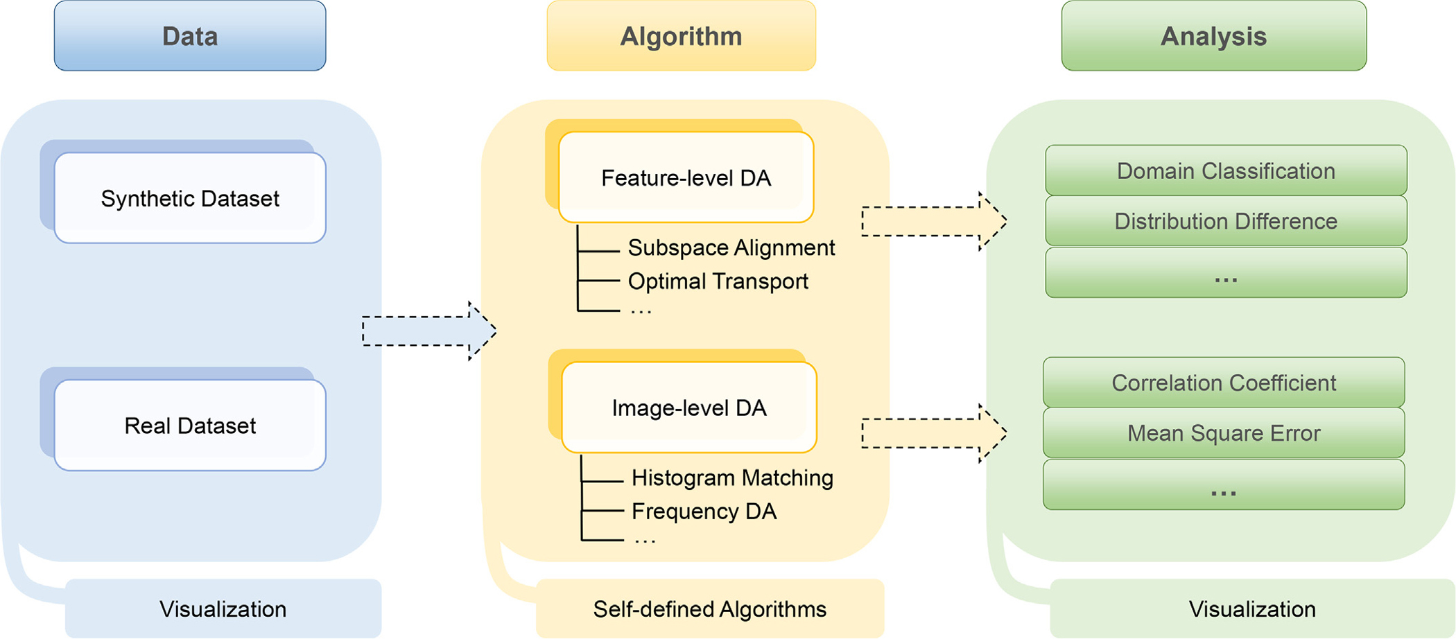
Illustration of workflow of the DomainATM software. The DomainATM consists of three major components: 1) the data module loads or creates the datasets; 2) the algorithm module conducts feature-level or image-level domain adaptation and saves the results; and 3) the evaluation module assesses the adaptation performance according to specific metrics. DA: Domain Adaptation.

The DomainATM is implemented in MATLAB (originally implemented in MATLAB 2021b on Windows 10, MATLAB 2019 or more advanced versions are all good for it). Through test, DomainATM can be run on Windows, Mac OS and Linux systems. It can be easily used with a graphical-user-interface (GUI), as shown in Fig. 3. The hardware platform can be a CPU-based PC (originally developed on Intel i-7 PC with 16 GB memory), which does not require much computation or memory resources. For advanced users, DomainATM provides an interface for writing MATLAB scripts to implement self-defined domain adaptation methods. The software, manual and source code for DomainATM are accessible online¹.

Fig. 3.

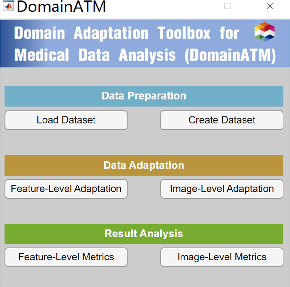
Graphical-User-Interface (GUI) of DomainATM.

3. Toolbox workflow

3.1. Creating/loading data

The DomainATM can work for both feature-level adaptation and image-level adaptation. These two key modules in the toolbox are independent of each other. With respect to the input of feature-level adaptation, the toolbox accepts data in standard MATLAB .mat file format. Each row represents an observation (subject or sample) while every column represents a feature. Existing real-world medical datasets (in .mat format) can be directly imported and loaded into the toolbox for processing. In addition, the users can create a synthetic dataset. After assigning the sample number, mean value and covariance matrix, the toolbox can automatically generate a synthetic dataset following a normal distribution. After loading the real/synthetic data, their distribution will be automatically displayed in the toolbox. Both the real-world and created datasets are stored in the “data” subfolder of the toolbox.

For image-level adaptation, the toolbox currently accepts 3D volumetric data (in .nii format). All the data will be converted to inner-built data in MATLAB. After loading the volumetric data, a middle slice (in axial view) will be automatically shown. Note that the “Create Dataset” module currently only generates data for feature-level domain adaptation.

3.2. Selecting domain adaptation algorithms

After loading the data, the following procedure is to select, configure, and run the domain adaptation methods. Most adaptation methods have several hyper-parameters to be set. Users can tune them according to the specific tasks. Otherwise, default settings of these methods will be used. After configuration, the users can run the algorithms. All the built-in methods provided by the toolbox are simple, easy to use, and can run in real time within 5 seconds (on a PC with an Intel i-7 CPU, 16 GB memory).

After running the adaptation methods, the results will be automatically saved in the “evaluation” subfolder of the toolbox. For feature-level adaptation, the original source/target data, and the adapted source/target data will be saved (in .mat data format). For image-level adaptation, the adapted source images (target image is used as the reference image and will not be changed) will be saved (in .nii format). All the files are named with the corresponding adaptation method with time stamp.

3.3. Evaluating data adaptation performance

After running the adaptation methods and getting the results, performance evaluation can be conducted for the methods. For feature-level adaptation, we use distribution difference and domain-level classification accuracy as two metrics to assess the adaptation performance. For image-level adaptation, we adopt correlation coefficient (CC), peak signal-to-noise ratio (PSNR) and mean-square error (MSE) to evaluate the adaptation result. More details about these evaluation metrics will be elaborated in the experiment section.

3.4. Visualization of data adaptation results

Besides quantitative evaluation, result visualization is useful for qualitative analysis. The DomainATM provides visualization functions that help users better understand domain adaptation for medical data. For feature-level adaption, the feature distribution (in 2D space) before and after adaptation can be visualized. High-dimensional features will be mapped to 2D feature space via t-SNE (Van der Maaten and Hinton, 2008). For image-level adaptation, the adapted source image, the original source and target images can be viewed using the toolbox. After the adapted images have been saved in the “evaluation” subfolder, they can also be visually inspected by other medical imaging software.

3.5. Extension: Adding self-defined data adaptation algorithm

In some tasks of medical data analysis, users might need to develop their own domain adaptation methods. The DomainATM supports self-defined algorithms for task-specific usage. The users can write a MATLAB script to define and implement their algorithms. The input/output format of the self-defined functions has to be consistent with other built-in adaptation methods. When adding an new algorithm, the self-defined script should be put in the “algorithms_feat” (feature-level) or the “algorithms_img” (image-level) subfolders in the toolbox. One can simply run and analyze their methods like the other built-in ones through GUI.

4. Algorithms

In this section, we briefly introduce the algorithms for feature-level and image-level data adaptation in DomainATM. More details can be found in the online manual.

4.1. Feature-level data adaptation algorithm

4.1.1. Baseline

No feature-level domain adaptation is utilized. Both source and target data are kept in their original distributions (in the feature space).

4.1.2. Subspace Alignment (SA)

In this algorithm (Fernando et al., 2013), the source and target medical data are represented by subspaces in terms of eigenvectors. The source data are projected to the target domain through a transformation matrix. No category labels of source domain are needed. The key hyper-parameter is the dimension of the shared subspace.

4.1.3. Correlation Alignment (CORAL)

In this algorithm (Sun et al., 2016), domain shift/difference is minimized by aligning the second-order statistics (e.g., covariance) of source and target distributions. No category label information and hyper-parameters are required for this method.

4.1.4. Transfer Component Analysis (TCA)

In this algorithm (Pan et al., 2010), a subspace shared by the source and target domain is searched in a reproducing kernel Hilbert space by minimizing the maximum mean discrepancy (MMD) distance. No source category labels are demanded. The key hyper-parameters are the kernel type and subspace dimension.

4.1.5. Optimal Transport (OT)

In this algorithm (Guan et al., 2021b), the samples in the source domain are projected into the target domain while keeping their conditional distributions. The projection is facilitated through minimization of Wasserstein distance between the two distributions. No category labels of the source domain are used. The key hyper-parameter is the regularization coefficient.

4.1.6. Joint Distribution Adaptation (JDA)

In this algorithm (Long et al., 2013), maximum mean discrepancy (MMD) is adopted to measure domain distribution differences, and is integrated into Principal Component Analysis (PCA) to build a representation that is robust to domain shift. Source category labels are needed in this algorithm. The key hyper-parameters include kernel type, subspace dimension and regularization parameter.

4.1.7. Transfer Joint Matching (TJM)

In this algorithm (Long et al., 2014), feature matching and instance reweighting strategies are combined to reduce domain shift. Minimization of maximum mean discrepancy (MMD) and l_2,1 norm sparsity penalty on source data are integrated into PCA to construct domain-invariant features. Category labels of source domain are required. The key hyper-parameters include kernel type, subspace dimension and regularization parameter.

4.1.8. Geodesic Flow Kernel (GFK)

In this algorithm (Gong et al., 2012), the source and target data are embedded into the Grassmann manifolds, and the geodesic flows between them are used to model domain shift. Domain adaptation is conducted by projecting the data into several domain-invariant subspaces on the geodesic flow. Source category labels can be either used or not. The key hyper-parameter is the subspace dimension.

4.1.9. Scatter Component Analysis (SCA)

In this algorithm (Ghifary et al., 2016), original features are firstly projected to a reproducing kernel Hilbert space. Domain adaptation is then conducted through an optimization formulation, including maximizing the class separability, maximizing the data separability, and minimizing domain mismatch. Category labels of the source domain are used during adaptation. The key parameter is the dimension of the transformed space.

4.1.10. Information-Theoretical Learning (ITL)

In this algorithm (Shi and Sha, 2012), an optimal feature space is learned through jointly maximizing domain similarity and minimizing the expected classification error on target samples. Source category labels are required. The key hyper-parameters include subspace dimension and regularization parameter.

4.2. Image-level data adaptation algorithm

4.2.1. Baseline

For two medical images acquired by different scanners/sites, no domain adaptation is facilitated in this method. Instead, the homogeneity/heterogeneity of the paired original images is directly compared in terms of certain evaluation metrics.

4.2.2. Histogram Matching (HM)

This method transforms source image to make its histogram matches the histogram of the target image (Shinohara et al., 2014). After adaptation, the intensity distributions of the source and target images become closer.

4.2.3. Spectrum Swapping-based Image-level MRI Harmonization (SSIMH)

In this method (Guan et al., 2022), the source and target images are firstly transformed into the frequency domain (e.g., through Discrete Cosine Transform). Then, part of the low-frequency region of source image is replaced by the corresponding low-frequency area of the target image. Finally, the source image in the revised frequency domain is inverted back to the spatial domain to get the adapted image. The key hyper-parameter of this method is the threshold which defines the low-frequency region that is swapped between source and target images. In the toolbox, the default value is set to 3.

The image-level domain adaptation methods work well in two different settings. (1) One-to-one image harmonization: Given a source image and a target/reference image, one can select a specific algorithm to adapt the source image to the target image space. (2) Batch image harmonization: Given multiple source images and a target image, we can adapt all source images to target image space via batch harmonization.

5. Empirical evaluation of feature-level data adaptation algorithms in DomainATM

5.1. Evaluation metric

For feature-level adaptation methods, we adopt the metrics that evaluate the distribution changes before and after the adaptation process. Specifically, we use the following three methods/metrics for adaptation performance evaluation.

• Distribution difference. We adopt maximum mean discrepancy (MMD) to measure the data distribution differences between the source and target domains before and after domain adaptation. As a popular metric, the maximum mean discrepancy (MMD) has been widely used in domain adaptation research (Kumagai and Iwata, 2019; Long et al., 2013; 2014; Pan et al., 2010; Wang et al., 2021; Yan et al., 2017), defined as follows:

  $$\mathbf{M}\mathbf{M}{\mathbf{D}}_k^2={\Vert {\mathbf{E}}_p\left[\varphi \left({\mathbf{x}}^s\right)\right]-{\mathbf{E}}_q\left[\varphi \left({\mathbf{x}}^t\right)\right]\Vert }_{{\mathscr{H}}_k}^2$$ (1)

  where ${\mathscr{H}}_k$ denotes the Reproducing Kernel Hilbert Space endowed with a kernel function k, and $k\left({\mathbf{x}}^s,{\mathbf{x}}^t\right)=\langle \varphi \left({\mathbf{x}}^s\right),\varphi \left({\mathbf{x}}^t\right)\rangle$. If the MMD distance of source and target domains gets lower after adaptation, it indicates the data distribution difference becomes smaller.

• Domain classification. Suppose an equal number of samples are sampled from the source and target domains, respectively. These samples are assigned with domain labels, i.e., the source samples are labeled as “1” while target samples are assigned with the label “0”. A domain discriminator/classifier is applied to all samples for distinguishing which samples come from the source domain and which ones are from the target domain. The classification result is used to assess domain shift/difference. A high domain classification accuracy indicates that the source and target samples can be easily distinguished, which means the domain shift is large. In contrast, if the domain classification accuracy drops down after the adaptation processing, it indicates the domain adaptation algorithm works because it makes the two domains get closer and become more difficult to distinguish.

5.2. Experiment 1: Adaptation on synthetic dataset

We first conduct experiments on synthetic datasets using DomainATM. Users can set the statistical properties of the synthetic data freely using DomainATM, and thus, can conduct fast test of different domain adaptation methods, which is helpful for understanding the characteristics of different methods and avoiding the access restrictions of many real-world medical datasets. Specifically, we generate two domains by Gaussian distributions. Each domain has two classes, with 30 positive samples and 30 negative ones, respectively. For the source domain $𝒮$, the means of positive and negative samples are [0, 0] and [0, 1], while their covariance matrices are [0.2, 0; 0, 0.2] and [0.1, 0; 0, 0.1]. For the target domain $𝒯$, the means of positive and negative samples are [1, −0.5] and [1, 0.2], while their covariance matrices are [0.2, 0; 0, 0.2] and [0.1, 0; 0, 0.1].

5.2.1. Data distribution visualization

The distributions of the original data and the adapted data by different methods are visualized in Fig. 4. From the visualization result, different domain adaptation methods can reduce the distributions of source and target samples to certain extent. For example, the optimal transport adaptation (OT) can project the source data into the target domain, and make the source distribution quite similar to the target domain.

Fig. 4.

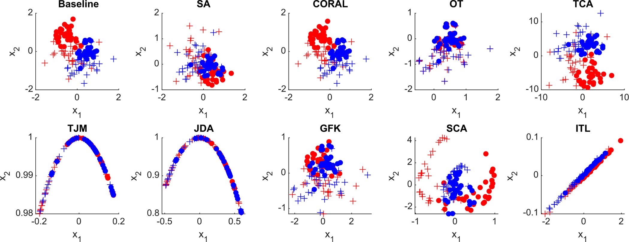
Distribution of the synthetic data (baseline) and adapted data by nine different domain adaptation methods in the DomainATM toolbox. (+ positive source samples; + positive target samples; • negative source samples; • negative target samples).

5.2.2. Distribution difference

The data distribution differences (in terms of maximum mean discrepancy) of the source and target domains after domain adaptation are shown in Fig. 5. The result of the Baseline method shows the original distribution of the source and target domain without any adaptation processing. From Fig. 5, we can observe that domain adaptation can reduce the distribution differences between the original source and target domains.

Fig. 5.

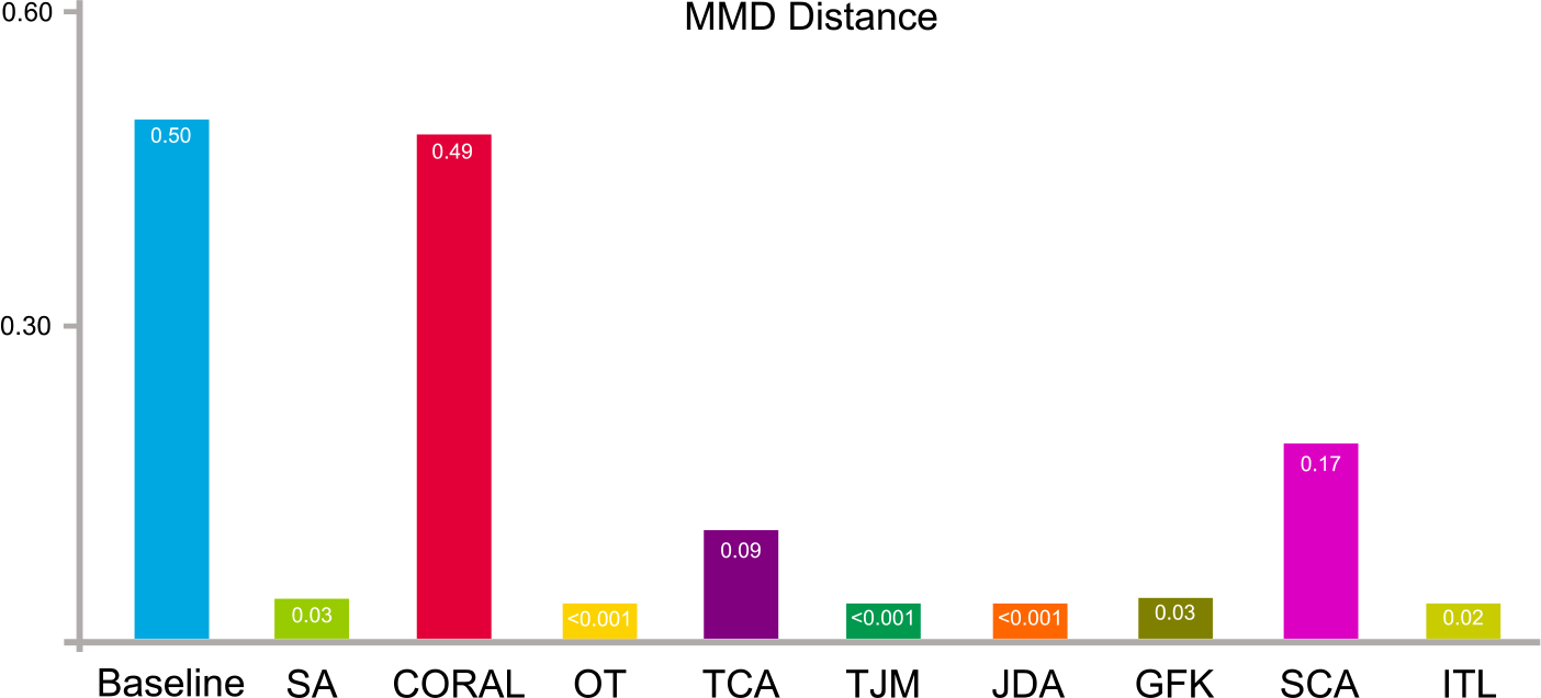
Synthetic data distribution differences in terms of maximum mean discrepancy before (baseline) and after domain adaptation using nine feature-level adaptation methods.

5.2.3. Domain-level classification

We conduct domain-level classification on the source and target data. A domain classifier (we use a k-nearest neighbors classifier) is trained with source data (with the label “1”) and target data (with the label “0”). Source and target data are combined together and shuffled. In the experiments, we use 60% of the entire data samples for training the domain classifier while 40% are for test. The result of domain classification accuracy is shown in Fig. 6.

Fig. 6.

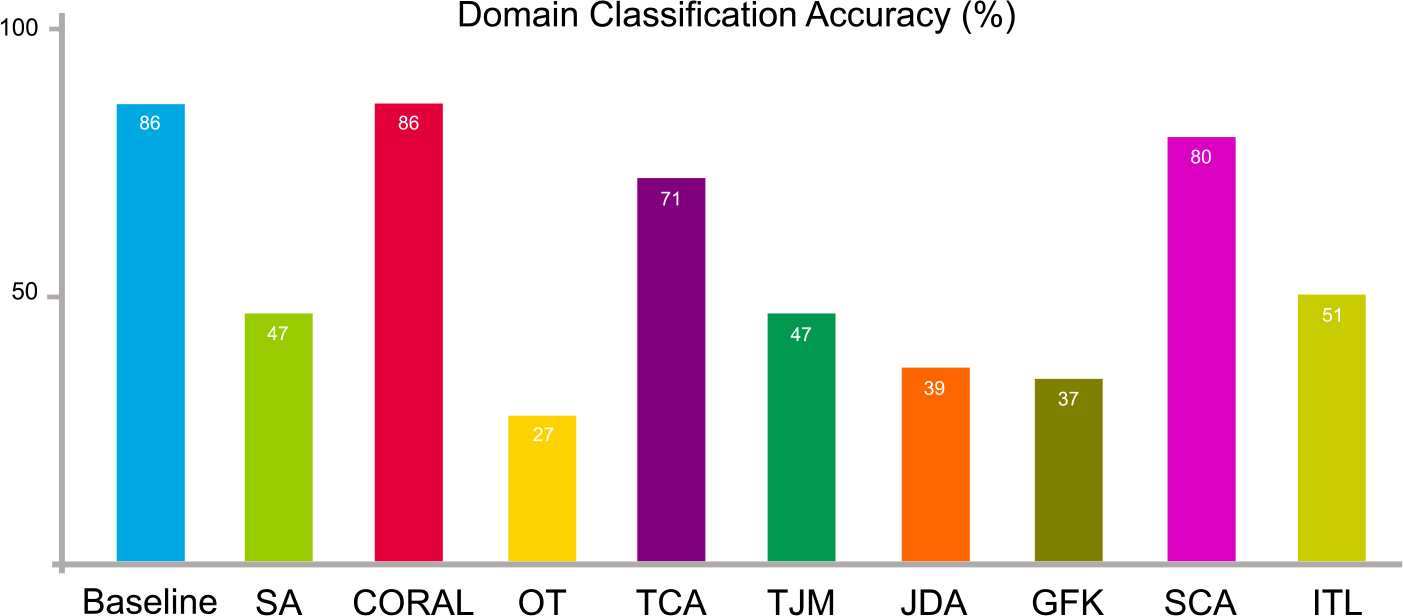
Synthetic data distribution differences in terms of domain-level classification accuracy on the synthetic dataset before (baseline) and after domain adaptation using nine feature-level adaptation methods.

We also use another two classifiers, i.e., support vector machine (SVM) and random forest (RF) for domain-level classification. For the SVM, we use a linear kernel and the penalty parameter C is set to 1. For the RF, 50 decision trees are used for the ensemble classification. These settings are also used for the other experiments. Their domain-level classification results are shown in Table 1.

Table 1.

Domain classification accuracy (%) using different classifiers on the synthetic dataset. (SVM: support vector machine; RF: random forest).

Method	Baseline	SA	CORAL	OT	TCA	TJM	JDA	GFK	SCA	ITL
SVM	85	47	80	35	77	40	41	39	60	41
RF	85	51	82	24	60	47	37	41	78	59

From Fig. 6 and Table 1, it can be seen that the domain classification accuracy drops after domain adaptation even different classifiers are used. This implies that source and target data become more difficult to be distinguished, i.e., domain adaptation makes their distributions become more similar than in the original space.

5.3. Experiment 2: Adaptation for Alzheimer’s disease analysis on ADNI

We conduct experiments on the Alzheimer’s Disease Neuroimaging Initiative (ADNI) dataset (Jack Jr et al., 2008). The dataset consists of T1-weighted MRI data for Alzheimer’s disease (AD) analysis. We use two subsets of ADNI, i.e., ADNI-1 (100 subjects with 1.5T T1-weighted structural MRIs) and ADNI-2 (100 subjects with 3.0T T1-weighted structural MRIs) as the source and target domains, respectively, to test the domain adaptation algorithms using DomainATM. ADNI-1 contains 50 patients with Alzheimer’s disease (AD) (positive samples) and 50 normal control (NC) subjects (negative samples). ADNI-2 has 50 CE subjects and 50 NC subjects. All the MRIs have been processed through a standard pipeline, including skull stripping, intensity correction, registration and re-sampling. Regions-of-interest (ROIs) features which are defined on 90 regions in the Anatomical Automatic Labeling (AAL) atlas (Tzourio-Mazoyer et al., 2002) are used to represent each subject. The 90-dimensional features denote the gray matter volumes in each brain region.

5.3.1. Distribution visualization

The distributions of original ADNI-1 and ADNI-2 data (in feature space) and the adapted data by different methods are visualized in Fig 7. From the visualization results, the original source and target data have a relatively clear boundary. After domain adaptation, the domain boundaries become blurred, and the distribution of source and target domains gets closer to each other.

Fig. 7.

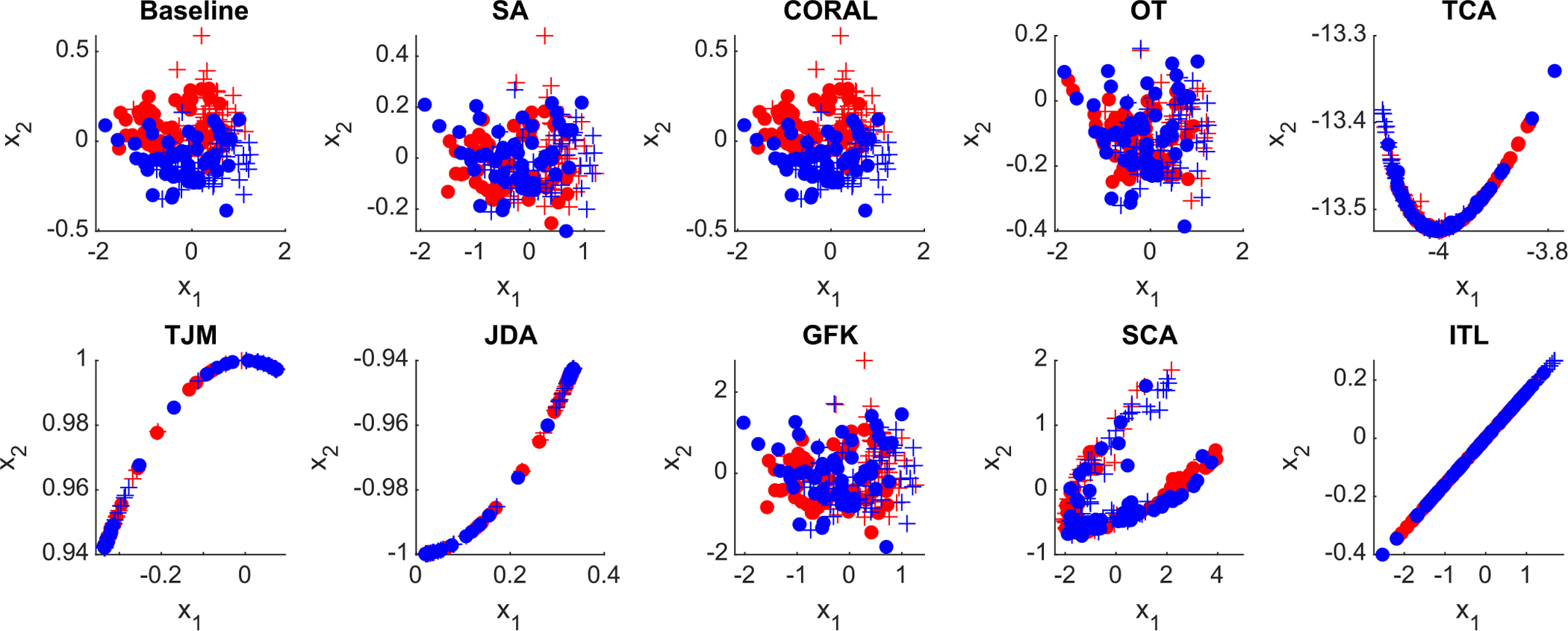
Distribution of the original ADNI data (baseline) and adapted data by nine feature-level domain adaptation methods in the DomainATM toolbox. (+ positive source samples; + positive target samples; • negative source samples; • negative target samples).

5.3.2. Distribution distance

The distribution differences (in terms of maximum mean discrepancy) of the source data, i.e., ADNI-1, and target data, i.e., ADNI-2, after domain adaptation are shown in Fig. 8. The baseline illustrates the original distribution of the source and target domain without any adaptation processing. From the result, it can be observed that domain adaptation is able to reduce the distribution differences between the original source and target domains.

Fig. 8.

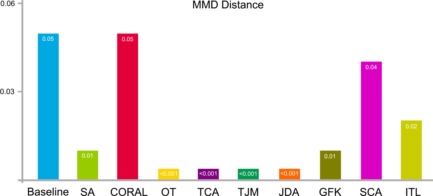
Data distribution differences in terms of maximum mean discrepancy on ADNI-1 and ADNI-2 before (baseline) and after domain adaptation operations.

5.3.3. Domain-level classification

We facilitate domain-level classification on the source data, i.e., ADNI-1, and target data, i.e., ADNI-2. A domain classifier (k-nearest neighbors classifier) is trained with source data (with the label “1”) and target data (with the label “0”). Source and target data are combined together and shuffled. 60% of the entire data are adopted for training while 40% for testing. The result of domain-level classification is illustrated in Fig. 9. Another two classifiers, including support vector machine (SVM) and random forest (RF) are also adopted for domain-level classification, and the result is listed in Table 2. From Fig. 9 and Table 2, we can see that the domain classification accuracy drops after domain adaptation despite the different types of domain classifiers. This indicates that the adapted source and target data get more difficult to be correctly classified, i.e., domain adaptation is effective in reducing their distribution differences.

Fig. 9.

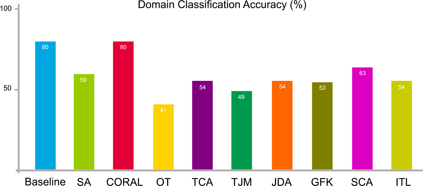
Data distribution differences in terms of domain-level classification accuracy on ADNI-1 and ADNI-2 before (baseline) and after domain adaptation operations.

Table 2.

Domain classification accuracy (%) using different classifiers on the ADNI-1 and ADNI-2 datasets. (SVM: support vector machine; RF: random forest).

Method	Baseline	SA	CORAL	OT	TCA	TJM	JDA	GFK	SCA	ITL
SVM	79	43	79	43	77	43	43	43	43	43
RF	85	64	85	52	80	63	58	60	50	57

5.4. Experiment 3: Domain adaptation for autism analysis on ABIDE

We conduct experiments on the Autism Brain Imaging Data Exchange (ABIDE) dataset (Di Martino et al., 2014). This database consists of resting-state functional MRI (fMRI) data for Autism analysis. We use two sites from the ABIDE project, i.e., NYU (184 subjects) and UM (145 subjects) as the source and target domains, respectively, to test the domain adaptation algorithms using the DomainATM. The NYU site consists of 79 positive samples (autism patients) and 105 negative samples (normal controls). These fMRIs are acquired by a 3 Tesla Allegra scanner. The UM site includes 68 positive samples (autism patients) and 77 negative samples (normal controls). These fMRIs are acquired using a 3 Tesla GE scanner located at the UM Functional MRI Laboratory. All the fMRIs go through a standard pipeline, including slice-timing and motion correction, nuisance signal regression, temporal filtering, and registration. The mean time series of 116 regions-of-interest (ROIs) defined by the Anatomical Automatic Labeling (AAL) atlas (Tzourio-Mazoyer et al., 2002) are extracted. Then, a 116×116 symmetrical resting-state functional connectivity (FC) matrix is generated for each subject, with each element representing the Pearson correlation coefficient between a pair of ROI signals. We extract the node betweenness centrality (Rubinov and Sporns, 2010) based on the FC matrix to represent each subject/sample.

5.4.1. Distribution visualization

The original distributions of two sites in ABIDE (in feature space) and the adapted data by different methods are visualized in Fig. 10. From the visualization result, it can be observed that the boundary between original source and target data is relatively clear. After the domain adaptation processing, the domain boundaries become blurred, and the distributions of source and target domain get similar to each other.

Fig. 10.

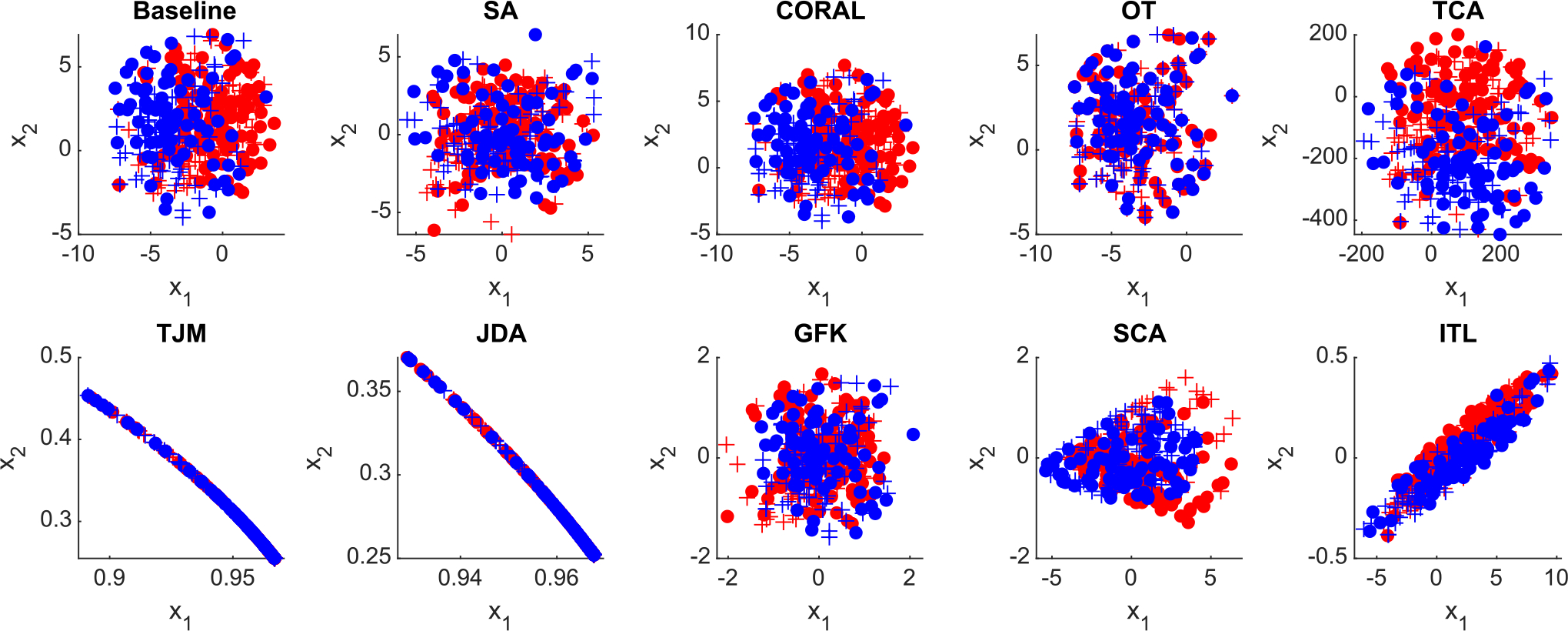
Distribution of the original ABIDE data (baseline) and adapted data by nine feature-level domain adaptation methods in the proposed DomainATM toolbox. (+ positive source samples; + positive target samples; • negative source samples; • negative target samples).

5.4.2. Distribution distance

The data distribution differences (in terms of MMD) of the source NYU domain and target UM domain after domain adaptation are shown in Fig. 11. The baseline is the original distribution of the source and target domain without any adaptation processing. The result shows that the distribution differences become smaller after adaptation processing by different algorithms.

Fig. 11.

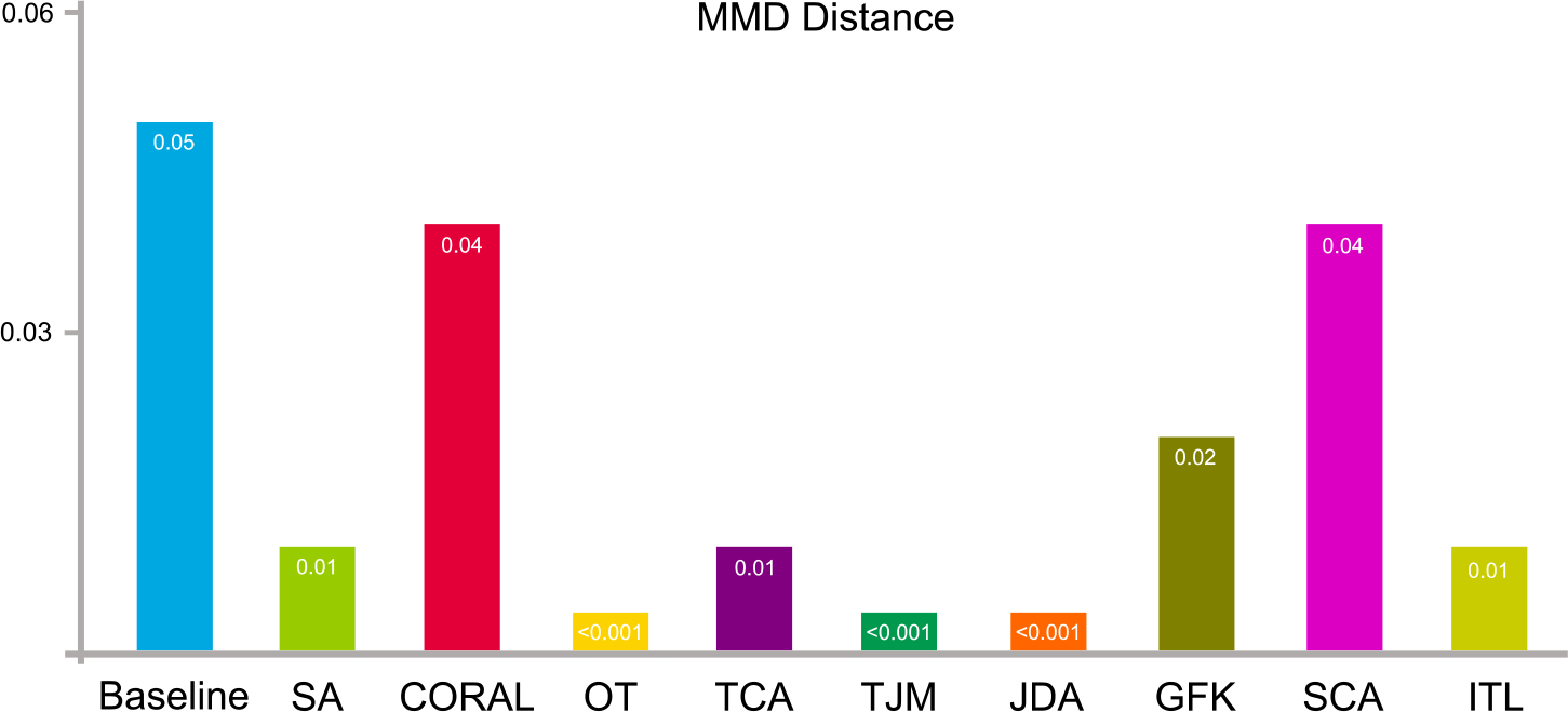
Data distribution differences of two sites of ABIDE in terms of maximum mean discrepancy before (baseline) and after domain adaptation using nine feature-level adaptation methods.

5.4.3. Domain-level classification

We facilitate domain-level classification on the source data, i.e., NYU, and target data, i.e., UM. A domain classifier (k-nearest neighbors classifier) is trained with source data (with the label “1”) and target data (with the label “0”). Source and target data are combined together and shuffled. 60% of the entire data are adopted for training while 40% for test. The result of domain-level classification accuracy is illustrated in Fig. 12. We also use support vector machine (SVM) and random forest (RF) to conduct the domain-level classification, and the result is shown in Table 3 From the results, the domain classification accuracy gets worse after domain adaptation processing regardless of what domain classifiers have been used. This indicates that the adapted source and target data become more difficult to be discriminated, i.e., using domain adaptation has successfully reduced their distribution differences.

Fig. 12.

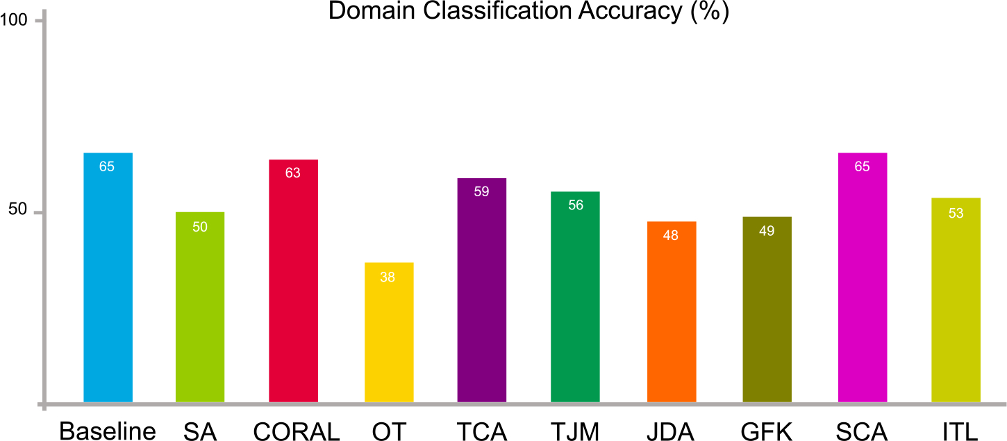
Data distribution differences in terms of domain-level classification accuracy on two sites of ABIDE before (baseline) and after domain adaptation using nine feature-level adaptation methods.

Table 3.

Domain classification accuracy (%) using different classifiers on two sites of ABIDE dataset. (SVM: support vector machine; RF: random forest).

Method	Baseline	SA	CORAL	OT	TCA	TJM	JDA	GFK	SCA	ITL
SVM	69	55	67	55	68	55	55	55	55	65
RF	66	55	64	31	66	48	43	50	65	63

5.5. Discussion

In the above experiments, we use two quantitative metrics, i.e., MMD and domain classification accuracy, to evaluate the performance of different domain adaptation methods in DomainATM. The MMD is a direct assessment metric because it is directly calculated based on the statistical properties of source and target domains (datasets). Generally, if method A achieves a smaller MMD than method B, then A is supposed to be better. Domain classification accuracy is an indirect metric because it relies on a specific domain classifier. But it can also reflect the adaptation performance since confusing a classifier is difficult. If method A achieves a smaller domain classification accuracy than method B, then A is supposed to be better. Based on the experimental results, we have the following empirical findings.

• The CORAL, TCA and SCA algorithms have relatively worse domain adaptation performance than the other methods. They get significantly higher MMD values and domain classification accuracy than the others.

• The OT algorithm achieves the overall best performance among these adaptation methods. It generally produces the smallest MMD value and domain classification accuracy in all these three experiments.

• On the ADNI dataset, the TJM, JDA, GFK and ITL have comparable performance. They get similar domain classification accuracy and low MMD. On the ABIDE dataset, the algorithm ITL is worse than the others.

• Most algorithms are effective in significantly reducing the MMD value. By contrast, the domain classification accuracy is more difficult to reduce. This implies that it is challenging to confuse or deceive a domain classifier with certain domain adaptation methods. Thus, domain classification accuracy is a rigorous metric to assess the robustness of an adaptation algorithm.

We also conduct statistical testing for performance comparison in terms of domain classification accuracy. Specifically, we compute the p-values via paired sample t-test between each adaptation method and the baseline. The p-values are smaller than 0.05, indicating that their differences are significant. In addition, we calculate the running time of each domain adaptation algorithm for each dataset on a PC with an Intel i-7 CPU and 16 GB memory. The comparison result is listed in Table 4.

Table 4.

Running time (in terms of seconds) of nine domain adaptation algorithms in DomainATM on three datasets.

Method	SA	CORAL	OT	TCA	TJM	JDA	GFK	SCA	ITL
Synthetic	0.09	0.05	1.28	0.06	0.19	0.85	0.09	1.04	0.06
ADNI	0.05	0.01	2.78	0.04	0.21	0.92	0.09	1.13	0.13
ABIDE	0.03	0.01	6.07	0.07	0.26	0.92	0.09	1.74	0.25

6. Empirical evaluation of image-level data adaptation algorithms in DomainATM

6.1. Evaluation metrics

For image-level adaptation methods, we adopt the metrics that evaluate the image similarity/dissimilarity before and after adaptation. Specifically, we adopt the following three metrics for image-level adaptation performance evaluation.

• Correlation Coefficient (CC). Denote the source and target images as ${ℐ}_s$ and ${ℐ}_t$. After adaptation, we get ${ℐ}_s^{\prime }$. For performance assessment, if the correlation coefficient of ${ℐ}_s^{\prime }$ and ${ℐ}_t$ is higher than ${ℐ}_s$ and ${ℐ}_t$, it indicates the corresponding adaptation algorithm works.

• Peak Signal-to-Noise Ratio (PSNR). If the peak signal-to-noise ratio of ${ℐ}_s^{\prime }$ and ${ℐ}_t$ is higher than ${ℐ}_s$ and ${ℐ}_t$, it indicates the adaptation algorithm works.

• Mean-Squared Error (MSE). If the mean-squared error of ${ℐ}_s^{\prime }$ and ${ℐ}_t$ is smaller than ${ℐ}_s$ and ${ℐ}_t$, it indicates the adaptation algorithms are effective.

6.2. Materials and settings

Phantom data of five traveling subjects with T1-weighted (T1-w) structural MRIs from the ABCD dataset (Volkow et al., 2018) are used for performance evaluation. Phantom-1 is scanned by GE and Philips scanners, respectively. Phantom-2 and Phantom-3 are acquired by Siemens and GE scanners, respectively. Phantom-4 and Phantom-5 are scanned by Philips and Siemens scanners, respectively. The protocols of the GE, Philips and Siemens scanners are consistent. These phantoms are used to test the performance of image-level domain adaptation methods in handling domain shift caused by different scanners. All these 3D MRIs are raw data in the NIfTI file format. We do not perform any pre-processing such as skull-stripping, registration or segmentation before image-level adaptation. During adaptation, the intensity of each image is normalized to the range of [0, 1]. For these volumetric images which contain multiple slices, the adaptation is facilitated on each slice, then the performance is calculated as an average metric value for all the slices within an image (volume).

6.3. Result

We conduct image-level domain adaptation on these five phantom structural MRI data, and the adaptation results in terms of the three metrics are shown in Table 5. From the result, it can be observed that image-level domain adaptation methods can generally achieve higher scores of correlation coefficient (CC) and peak signal-to-noise ratio (PSNR) and smaller mean square error (MSE). In some cases (e.g., GE → Philips), the Histogram Matching (HM) does not perform very well in terms of PSNR and MSE. Overall, the result indicates that image-level adaptation methods are useful in reducing the distribution shift between images caused by different scanners.

Table 5.

Results of three image-level domain adaptation methods on T1-weighted MRIs of five traveling phantom subjects acquired by three different scanners from the ABCD dataset.

Source Domain→Target Domain (Subject ID)	Method	CC	PSNR	MSE
G→Siemens (Phantom-2, Phantom-3)	Baseline	0.4889±0.0081	21.4143± 2.8718	0.0080± 0.0049
	HM	0.5642±0.0395	22.3131± 2.5975	0.0064± 0.0037
	SSIMH	0.5935±0.0221	22.7624± 2.5310	0.0057± 0.0032
Philips→iemens	Baseline	0.5408±0.0194	18.7578± 0.8847	0.0135± 0.0028
(Phantom-4, Phantom-5)	HM	0.5495±0.0388	18.7477± 1.1303	0.0135± 0.0035
	SSIMH	0.6098±0.0269	20.1269± 1.8421	0.0101± 0.0042
GE→Philips (Phantom-1)	Baseline	0.4682	21.3915	0.0073
	HM	0.5108	21.2482	0.0075
	SSIMH	0.5570	22.6421	0.0054

6.4. Visual inspection

To further investigate the effectiveness of image-level domain adaptation, we do visual inspections of the MRIs that are adapted to different scanner styles. We divide the phantom MRIs into three groups in terms of the scanners. Then we adapt MRIs acquired by one scanner to the styles of MRIs scanned by other scanners. We use the SSIMH method (Guan et al., 2022) in DomainATM to perform image-level adaptation. Fig. 13 shows the results of three different MRIs and their corresponding adapted images to different scanner styles. From the result, we have the following two observations. 1) Different scanners (i.e., Siemens, Philips and GE) have a significant impact on the MRIs, which can cause the domain shift. 2) The image-level domain adaptation method is effective in harmonizing the source image to the target image (reference image) and reducing the domain shift caused by different scanners.

Fig. 13.

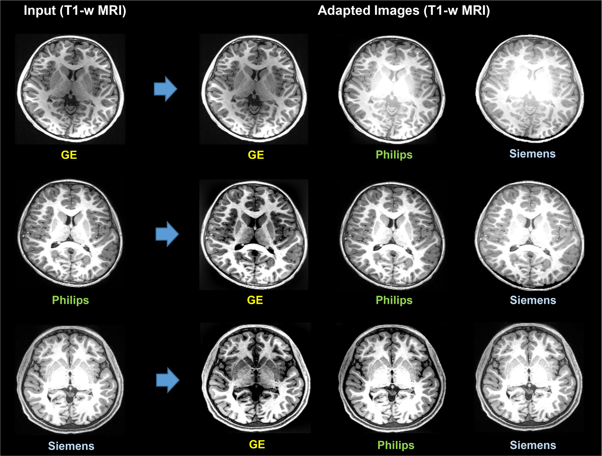
Image-level domain adaptation via the Spectrum Swapping-based Image-level MRI Harmonization (SSIMH) method (Guan et al., 2022) for T1-weighted (T1-w) MRIs acquired by different scanners. Domain shift caused by the use of different scanners can be partly reduced by image-level adaptation via SSIMH.

7. Conclusion and future work

Domain adaptation has become an important topic in the field of medical data analysis. In this paper, we develop a Domain Adaptation Toolbox for Medical data analysis (DomainATM), aiming to help researchers facilitate fast domain adaptation for medical data acquired from different sites/scanners. The DomainATM is easy to use, efficient to run, and most importantly, it is able to do both feature-level and image-level adaptation. In addition, users can add their own domain adaptation algorithms into the toolbox, making it flexible and extensible. Experiments on both synthetic and real-world medical datasets have been conducted to show the usage and effectiveness of DomainATM. We hope the toolbox can provide more convenience and benefit for researchers to do domain adaptation research in medical data analysis.

There are several potential future works to further enrich and extend the DomainATM. First, for the sake of fast and easy facilitation of domain adaptation in medical imaging data, we only include machine learning methods in the current version, without considering deep learning methods that often require large computation resources. In the future, we plan to develop another version of the toolbox to include deep learning methods (such as various GANs (Sinha et al., 2021; Yi et al., 2019) and CNNs (Guan et al., 2021a; Tibrewala et al., 2020)). Second, the current evaluation metrics merely reflect domain differences, lacking the ability to further analyze practical applications (e.g., to what extent Dice scores in a segmentation application varies before and after domain adaptation). We will address this issue to enrich the toolbox in the future. Besides, we plan to further improve the graphic user interface to enable users to set and tune the hyper-parameters of each domain adaptation method in a more convenient manner.

Fig. 1.

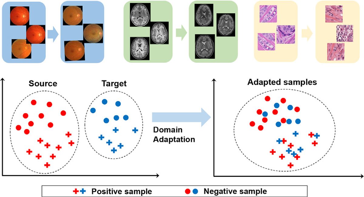
Illustration of the “domain shift” phenomenon (Quiñonero-Candela et al., 2009) (top row) and the fundamental of domain adaptation (distribution of source and target samples before and after adaptation).

Data Availability

The ADNI dataset used in this study can be accessed via the following link http://www.ida.loni.usc.edu/login.jsp?project=ADNI&page=HOME. An access application should be permitted firstly.

The ABIDE dataset used in this study can be accessed via the following link http://www.fcon_1000.projects.nitrc.org/indi/abide/abide_I.html. An access application should be permitted firstly.

For review convenience, we included the processed datasets (in terms of 2D features) in the submitted source code of this paper which can be found in the data folder.

References

- Barragán-Montero, et al. , 2021. Artificial intelligence and machine learning for medical imaging: a technology review. Physica Med. 83, 242–256. [DOI] [PMC free article] [PubMed] [Google Scholar]
- Ben-David S, Blitzer J, Crammer K, Pereira F, et al. , 2007. Analysis of representations for domain adaptation. MIT; 1998, pp. 137–144. [Google Scholar]
- Csurka G, 2017. A comprehensive survey on domain adaptation for visual applications. In: Domain Adaptation in Computer Vision Applications. Springer, pp. 1–35. [Google Scholar]
- Deo RC, 2015. Machine learning in medicine. Circulation 132 (20), 1920–1930. [DOI] [PMC free article] [PubMed] [Google Scholar]
- Di Martino A, Yan CG, Li Q, Denio E, et al. , 2014. The autism brain imaging data exchange: towards a large-scale evaluation of the intrinsic brain architecture in autism. Mol. Psychiatry 19 (6), 659–667. [DOI] [PMC free article] [PubMed] [Google Scholar]
- Erickson BJ, Korfiatis P, Akkus Z, Kline TL, 2017. Machine learning for medical imaging. Radiographics 37 (2), 505. [DOI] [PMC free article] [PubMed] [Google Scholar]
- Fatima M, Pasha M, et al. , 2017. Survey of machine learning algorithms for disease diagnostic. Journal of Intelligent Learning Systems and Applications 9 (01), 1. [Google Scholar]
- Fernando B, Habrard A, Sebban M, Tuytelaars T, 2013. Unsupervised visual domain adaptation using subspace alignment. In: Proceedings of the IEEE International Conference on Computer Vision, pp. 2960–2967. [Google Scholar]
- Ghifary M, Balduzzi D, Kleijn WB, Zhang M, 2016. Scatter component analysis: a unified framework for domain adaptation and domain generalization. IEEE Trans Pattern Anal Mach Intell 39 (7), 1414–1430. [DOI] [PubMed] [Google Scholar]
- Gong B, Shi Y, Sha F, Grauman K, 2012. Geodesic flow kernel for unsupervised domain adaptation. In: 2012 IEEE Conference on Computer Vision and Pattern Recognition. IEEE, pp. 2066–2073. [Google Scholar]
- Guan H, Liu M, 2022. Domain adaptation for medical image analysis: asurvey. IEEE Trans. Biomed. Eng. 69 (3), 1173–1185. [DOI] [PMC free article] [PubMed] [Google Scholar]
- Guan H, Liu S, Lin W, Yap P-T, Liu M, 2022. Fast image-level MRI harmonization via spectrum analysis. International Workshop on Machine Learning in Medical Imaging. Springer. [DOI] [PMC free article] [PubMed] [Google Scholar]
- Guan H, Liu Y, Yang E, Yap P-T, Shen D, Liu M, 2021. Multi-site MRI harmonization via attention-guided deep domain adaptation for brain disorder identification. Med Image Anal 71, 102076. [DOI] [PMC free article] [PubMed] [Google Scholar]
- Guan H, Wang L, Liu M, 2021. Multi-source domain adaptation via optimal transport for brain dementia identification. In: 2021 IEEE 18th International Symposium on Biomedical Imaging (ISBI). IEEE, pp. 1514–1517. [Google Scholar]
- Jack CR Jr, Bernstein MA, Fox NC, et al. , 2008. The Alzheimer’s Disease Neuroimaging Initiative (ADNI): MRI methods. J. Magn. Reson. Imaging 27 (4), 685–691. [DOI] [PMC free article] [PubMed] [Google Scholar]
- Kondrateva E, Pominova M, Popova E, Sharaev M, Bernstein A, Burnaev E, 2021. Domain shift in computer vision models for MRI data analysis: An overview. In: Thirteenth International Conference on Machine Vision, Vol. 11605. SPIE, pp. 126–133. [Google Scholar]
- Kouw WM, Loog M, 2019. A review of domain adaptation without target labels. IEEE Trans Pattern Anal Mach Intell 43 (3), 766–785. [DOI] [PubMed] [Google Scholar]
- Kumagai A, Iwata T, 2019. Unsupervised domain adaptation by matching distributions based on the maximum mean discrepancy via unilateral transformations. In: Proceedings of the AAAI Conference on Artificial Intelligence, Vol. 33, pp. 4106–4113. [Google Scholar]
- Lee H, Nakamura K, Narayanan S, Brown RA, Arnold DL, Initiative ADN, et al. , 2019. Estimating and accounting for the effect of MRI scanner changes on longitudinal whole-brain volume change measurements. Neuroimage 184, 555–565. [DOI] [PubMed] [Google Scholar]
- Long M, Wang J, Ding G, Sun J, Yu PS, 2013. Transfer feature learning with joint distribution adaptation. In: Proceedings of the IEEE International Conference on Computer Vision, pp. 2200–2207. [Google Scholar]
- Long M, Wang J, Ding G, Sun J, Yu PS, 2014. Transfer joint matching for unsupervised domain adaptation. In: Proceedings of the IEEE Conference on Computer Vision and Pattern Recognition, pp. 1410–1417. [Google Scholar]
- Van der Maaten L, Hinton G, 2008. Visualizing data using t-SNE. Journal of Machine Learning Research 9 (11). [Google Scholar]
- Pan SJ, Tsang IW, Kwok JT, Yang Q, 2010. Domain adaptation via transfer component analysis. IEEE Trans. Neural Networks 22 (2), 199–210. [DOI] [PubMed] [Google Scholar]
- Patel VM, Gopalan R, Li R, Chellappa R, 2015. Visual domain adaptation: a survey of recent advances. IEEE Signal Process Mag 32 (3), 53–69. [Google Scholar]
- Pooch EH, Ballester P, Barros RC, 2020. Can we trust deep learning based diagnosis? The impact of domain shift in chest radiograph classification. In: International Workshop on Thoracic Image Analysis. Springer, pp. 74–83. [Google Scholar]
- Quiñonero-Candela J, Sugiyama M, Lawrence ND, Schwaighofer A, 2009. Dataset Shift in Machine Learning. MIT Press. [Google Scholar]
- Rajkomar A, Dean J, Kohane I, 2019. Machine learning in medicine. N top N. Engl. J. Med. 380 (14), 1347–1358. [DOI] [PubMed] [Google Scholar]
- Rubinov M, Sporns O, 2010. Complex network measures of brain connectivity: uses and interpretations. Neuroimage 52 (3), 1059–1069. [DOI] [PubMed] [Google Scholar]
- Shi Y, Sha F, 2012. Information-theoretical learning of discriminative clusters for unsupervised domain adaptation. In: Proceedings of the 29th International Conference on International Conference on Machine Learning, pp. 1275–1282. [Google Scholar]
- Shinohara RT, et al. , 2014. Statistical normalization techniques for magnetic resonance imaging. NeuroImage: Clinical 6, 9–19. [DOI] [PMC free article] [PubMed] [Google Scholar]
- Sinha S, Thomopoulos SI, Lam P, Muir A, Thompson PM, 2021. Alzheimer’s disease classification accuracy is improved by MRI harmonization based on attention-guided generative adversarial networks. In: 17th International Symposium on Medical Information Processing and Analysis, Vol. 12088. SPIE, pp. 180–189. [DOI] [PMC free article] [PubMed] [Google Scholar]
- Sun B, Feng J, Saenko K, 2016. Return of frustratingly easy domain adaptation. In: Proceedings of the AAAI Conference on Artificial Intelligence, Vol. 30. [Google Scholar]
- Tibrewala R, Ozhinsky E, Shah R, Flament I, Crossley K, Srinivasan R, Souza R, Link TM, Pedoia V, Majumdar S, 2020. Computer-aided detection AI reduces interreader variability in grading hip abnormalities with MRI. J. Magn. Reson. Imaging 52 (4), 1163–1172. [DOI] [PMC free article] [PubMed] [Google Scholar]
- Torralba A, Efros AA, 2011. Unbiased look at dataset bias. In: Proceedings of the IEEE Conference on Computer Vision and Pattern Recognition. IEEE, pp. 1521–1528. [Google Scholar]
- Tzourio-Mazoyer N, et al. , 2002. Automated anatomical labeling of activations in SPM using a macroscopic anatomical parcellation of the MNI MRI single-subject brain. Neuroimage 15 (1), 273–289. [DOI] [PubMed] [Google Scholar]
- Valiant LG, 1984. A theory of the learnable. Commun ACM 27 (11), 1134–1142. [Google Scholar]
- Valverde JM, Imani V, Abdollahzadeh A, De Feo R, Prakash M, Ciszek R, Tohka J, 2021. Transfer learning in magnetic resonance brain imaging: a systematic review. Journal of Imaging 7 (4), 66. [DOI] [PMC free article] [PubMed] [Google Scholar]
- Volkow ND, et al. , 2018. The conception of the ABCD study: from substance use to a broad NIH collaboration. Dev Cogn Neurosci 32, 4–7. [DOI] [PMC free article] [PubMed] [Google Scholar]
- Wang M, Deng W, 2018. Deep visual domain adaptation: a survey. Neurocomputing 312, 135–153. [Google Scholar]
- Wang W, Li H, Ding Z, Nie F, Chen J, Dong X, Wang Z, 2021. Rethinking maximum mean discrepancy for visual domain adaptation. IEEE Trans Neural Netw Learn Syst. [DOI] [PubMed] [Google Scholar]
- Wilson G, Cook DJ, 2020. A survey of unsupervised deep domain adaptation. ACM Transactions on Intelligent Systems and Technology (TIST) 11 (5), 1–46. [DOI] [PMC free article] [PubMed] [Google Scholar]
- Wittens MMJ, et al. , 2021. Inter-and intra-scanner variability of automated brain volumetry on three magnetic resonance imaging systems in Alzheimer’s disease and controls. Front Aging Neurosci 13. [DOI] [PMC free article] [PubMed] [Google Scholar]
- Yan H, Ding Y, Li P, Wang Q, Xu Y, Zuo W, 2017. Mind the class weight bias: Weighted maximum mean discrepancy for unsupervised domain adaptation. In: Proceedings of the IEEE Conference on Computer Vision and Pattern Recognition, pp. 2272–2281. [Google Scholar]
- Yi X, Walia E, Babyn P, 2019. Generative adversarial network in medical imaging: a review. Med Image Anal 58, 101552. [DOI] [PubMed] [Google Scholar]
- Zhang J, Chao H, Yan P, 2020. Robustified domain adaptation. arXiv: 2011.09563 [Google Scholar]
- Zou D, Zhu Q, Yan P, 2020. Unsupervised domain adaptation with dual-scheme fusion network for medical image segmentation. In: International Joint Conference on Artificial Intelligence, pp. 3291–3298. [Google Scholar]
Associated Data
This section collects any data citations, data availability statements, or supplementary materials included in this article.
Supplementary Materials
Data Availability Statement